Figure
1.
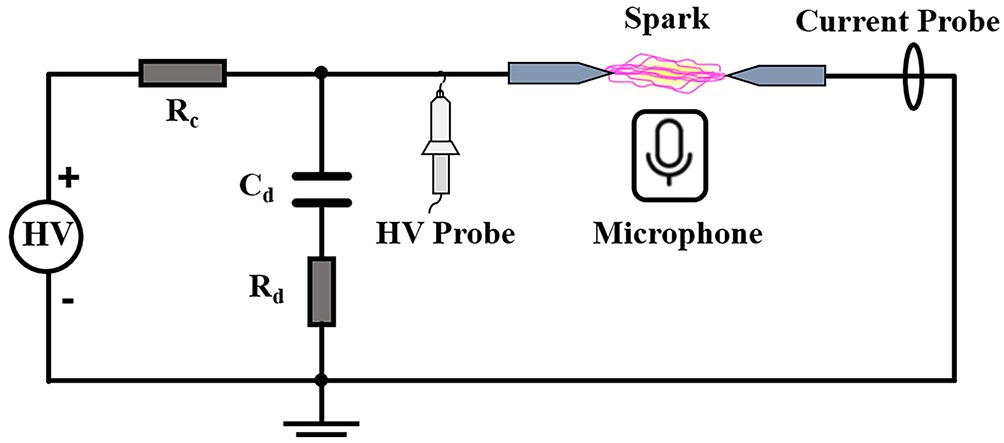
Schematic diagram of the experimental setup.
| Citation: |
Jun XIONG, Shiyu LU, Xiaoming LIU, Wenjun ZHOU, Xiaoming ZHA, Xuekai PEI. Machine learning for parameters diagnosis of spark discharge by electro-acoustic signal[J]. Plasma Science and Technology, 2024, 26(8): 085403. DOI: 10.1088/2058-6272/ad495e

|
Discharge plasma parameter measurement is a key focus in low-temperature plasma research. Traditional diagnostics often require costly equipment, whereas electro-acoustic signals provide a rich, non-invasive, and less complex source of discharge information. This study harnesses machine learning to decode these signals. It establishes links between electro-acoustic signals and gas discharge parameters, such as power and distance, thus streamlining the prediction process. By building a spark discharge platform to collect electro-acoustic signals and implementing a series of acoustic signal processing techniques, the Mel-Frequency Cepstral Coefficients (MFCCs) of the acoustic signals are extracted to construct the predictors. Three machine learning models (Linear Regression, k-Nearest Neighbors, and Random Forest) are introduced and applied to the predictors to achieve real-time rapid diagnostic measurement of typical spark discharge power and discharge distance. All models display impressive performance in prediction precision and fitting abilities. Among them, the k-Nearest Neighbors model shows the best performance on discharge power prediction with the lowest mean square error (MSE = 0.00571) and the highest R-squared value (R2=0.93877). The experimental results show that the relationship between the electro-acoustic signal and the gas discharge power and distance can be effectively constructed based on the machine learning algorithm, which provides a new idea and basis for the online monitoring and real-time diagnosis of plasma parameters.
In the past two decades, plasma has been widely used in various fields due to its high chemical activity, such as bio-medicine [1–5], auxiliary combustion [6–8], environmental governance [9], flow control [10], material processing, and material synthesis [11, 12]. Plasma boasts extensive applications but faces challenges due to environmental disturbances and the inherent sensitivity of its sources during generation. This sensitivity leads to high instability, complicating research and practical applications. Consequently, real-time monitoring of plasma parameters becomes crucial. It enables a deeper understanding and more effective control of plasma characteristics and effects. Furthermore, it aids in fulfilling real-world needs, including dependable operation across diverse applications. This is particularly vital in plasma medicine, where handheld devices demand ease of use and instant adaptability, all while ensuring safety and reliability during operation. Therefore, the real-time monitoring of plasma parameters holds significant practical value. In addition, plasma also has wide application prospects in substance synthesis and material processing, such as nitrogen fixation technology, material coating treatment, and disinfection treatment. In order to evaluate its energy utilization efficiency and the stability of injected power, the real-time prediction of discharge power is also an important factor to ensure stable and efficient operation.
At present, the commonly used diagnostic methods of plasma mainly include laser-induced fluorescence, mass spectrometry, spontaneous raman scattering, optical emission spectroscopy(OES), and instantaneous state voltage and current methods, among others [13–17]. These methods often have high requirements for instruments or test devices, which are unfavorable for real-time diagnosis of plasma. Compared with these complex diagnostic methods, the acoustic signal contained in the discharge process can be collected with just a microphone. Sound recognition (electro-acoustic signal) offers the advantages of being non-contact, having a small collector size, convenient installation, and easy signal acquisition, which is more conducive to simplifying plasma diagnostic equipment. According to the gas discharge mechanism, there is a certain relationship between the acoustic wave parameters and the discharge parameters [18–20], but this relationship is implicit, and the measured sound signal cannot directly reflect the real-time physical quantity. Establishing a connection between such indirect information and physical quantity parameters is challenging, requiring extensive calculations and analyses to form the relationship. This study aims to leverage machine learning algorithms to map the relationship between acoustic signals and discharge power and distance. By analyzing vast datasets with machine learning techniques, it seeks to identify correlations between sound signals and discharge parameters. The goal is to derive statistical sound signal characteristics for these parameters, enabling the prediction of unknown discharge parameters for new data points.
Research on predicting and diagnosing discharge plasma parameters using machine learning or artificial intelligence methods has attracted widespread attention [21–23]. In 2020, Sibanyoni et al [24] employed acoustic measurement instruments to diagnose a corona discharge device driven by high-voltage direct current. Through machine learning data measurement methods, they established a relationship between the discharge gap distance and electro-acoustic signals, achieving real-time online detection of discharge distances. Shojaei and Mangolini [25] discussed the use of probabilistic deep neural networks for the prediction of the electron energy probability function in low-temperature non-thermal plasmas and found that Bayesian models are preferable as they assign a higher level of uncertainty to their prediction especially when the dataset used to train them is small. This work describes one of the many potential applications of machine learning in plasma science and technology. It is found that Bayesian models are preferable as they assign a higher level of uncertainty to their prediction especially when the dataset used to train them is small. This work describes one of the many potential applications of machine learning in plasma science and technology. Gidon et al [26] introduced a novel deep learning-assisted, non-invasive method using microwave-plasma interactions to accurately estimate electron density profiles in low-temperature plasmas, overcoming limitations of conventional methods and demonstrating promising results in plasma diagnostics through comprehensive simulations and evaluations. Chang et al [27] demonstrated the effective use of a convolutional neural network, specifically the InceptionTime model, for real-time classification and analysis of atmospheric-pressure plasma jet currents, achieving high accuracy in identifying working gases and discharge types, and showcasing the potential for rapid monitoring and diagnosis in plasma applications. Zhang et al [28] presented a neural network model for real-time monitoring and feedback control of a miniaturized ion thruster's performance, using optical emission spectroscopy to accurately relate grid voltage and extraction current, achieving less than 6% deviation from experimental values and promising improvements for precise thrust control in space-based gravitational wave detection.
Current research on using electro-acoustic signals and machine learning methods for predicting discharge plasma parameters is relatively scarce. This paper focuses on utilizing a discharge platform to collect electro-acoustic signals and performing a series of audio signal processing to extract features for constructing criteria. By integrating various machine learning algorithms, the study successfully achieves real-time and rapid diagnostic measurement of a typical spark discharge power and discharge distance.
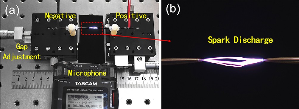
Figure 1 shows the schematic diagram of the experimental setup. A high-voltage DC power supply, the Spellman SL10PN1200, with a power capacity of 1200 W and a maximum output voltage of 10 kV, is utilized to charge the capacitor Cd, subsequently discharging to generate repetitive frequency sparks. By adjusting the Cd value, the charging time can be changed, which in turn alters the spark discharge frequency. In this study, we applied three different capacitance values which are 250 pF, 510 pF, and 1000 pF, respectively. The capacitors are chosen to cover a broad range of capacitances to explore how the capacitance affects the spark discharge frequency and the charging time. In the circuit, Rc is the charging resistor (2 MΩ) and Rd is the discharge resistor (200 Ω). The selection of a 2 MΩ charging resistor ensures that the capacitor charges at a controlled rate, preventing too rapid charging that could lead to equipment damage or inconsistent discharges. The 200 Ω discharge resistor is chosen to limit the current pulse peaks during discharge, reducing the risk of damaging the electrodes or affecting the discharge’s stability. These values balance between efficient charging and safe, controlled discharges. The discharge electrode is made of 2 identical stainless steel needles. Their length is 55 mm, diameter is 1.6 mm, and radius of tip curvature is 50 μm. The electrodes are fixed on two precision micrometer stages using nylon pillars for insulation, each pillar being 25 mm high and 8 mm in diameter. The position of the stages is adjusted to ensure that both electrodes are horizontal and coaxial. The distance between the tips of the electrodes can be precisely adjusted, with a range of 0–5 mm in the experiments.
When an appropriate high-voltage DC is applied, repetitive spark discharges occur across the discharge gap, as shown in the physical diagram of the experimental setup and the photo of spark discharge in figure 2. To capture the sound signal produced by the spark discharge, a microphone (Tascam DR-100mkII) is placed 50 mm away from the discharge gap. In the experiments, after stabilizing the discharge, the discharge sound signal is recorded for about 5 s under each experimental condition. Additionally, to obtain the discharge power characteristics of the spark discharge, the discharge voltage and current across the discharge gap are synchronously measured using a high-voltage probe (Tektronix, P6015A) and a current probe (Pearson, 2877). The measurement positions are shown in figure 1. The data collected by the high-voltage and current probes are displayed and saved using an oscilloscope (Tektronix, TBS2204B). The discharge power is calculated using the following formula after obtaining the data on discharge voltage and current.
| Pdis=f∫τ0V(t)I(t)dt. | (1) |
Here, f is the discharge frequency, V(t) is the discharge voltage, I(t) is the discharge current and τ is the discharge pulse-width.
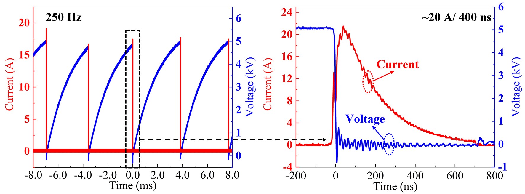
The typical discharge voltage and current waveform are shown in figure 3. The experimental conditions include a capacitance (Cd) of 1000 pF, an applied voltage (Va) of 7.5 kV, and a specific electrode tip gap distance of 4 mm. The left figure shows the waveform over several discharge cycles, with the blue line representing the discharge voltage and the red line representing the discharge current. The discharge appears stable, with a frequency of about 250 Hz. Within one discharge cycle, the charging time for Cd is about 4 ms. When the voltage across Cd reaches the gap breakdown voltage of 5 kV, the gap breaks down, resulting in a spark discharge that forms a short pulse current, accompanied by an electro-acoustic signal. The right figure is a magnified partial view of the voltage and current waveform at the moment of gap breakdown. We can see that the voltage across the electrodes drops rapidly to a minimal value and oscillates. The discharge current quickly peaks at about 22 A, then gradually decays to zero, with a half-peak width of the current pulse of about 300 ns.
To collect data on the sounds produced by spark discharges under different conditions, we have set three types of variable parameters: capacitor size (Cd) with values of 250 pF, 510 pF, 1000 pF; gap distance (d) at 1.0 mm, 1.5 mm, 2.0 mm, 2.5 mm, 3.0 mm, 3.5 mm, 4.0 mm, 4.5 mm, 5.0 mm; and applied voltage (Va) at 4.5 kV, 5.0 kV, 5.5 kV, 6.0 kV, 6.5 kV, 7.0 kV, 7.5 kV, 8.0 kV, 8.5 kV, 9.0 kV, 9.5 kV. The discharge power for each condition can be seen in the attached data.
In this study, we choose three different models, including Linear Regression, k-Nearest Neighbors, and Random Forest, to implement the training and prediction processes. For the theory and details of these models, we can refer to the following references [29–34]. Here is a brief introduction to these models.
Linear regression can be thought as applying a linear relationship between the input features of each data point and its corresponding output labels, shown as:
| y=β0+β1x+e, | (2) |
where x is the input data with one feature, β0 is the intercept, β1 is the slope, and e is the error between the real y and predicted ˆy. When the input data has n data points, each has multiple features, the above one-feature expression can be rewritten in a matrix form:
| y=Xβ+e, | (3) |
with {\boldsymbol{y}} = \begin{bmatrix} y_1 \\ y_2 \\ \vdots \\ y_n \end{bmatrix} , {\boldsymbol{X}} = \begin{bmatrix} 1 & x_{11} & \dots & x_{1p}\\ 1 & x_{21} & \dots & x_{2p} \\ \dots & \dots & \dots & \dots \\ 1 & x_{n1} & \dots & x_{np} \end{bmatrix} , and {\boldsymbol{\beta}} = \begin{bmatrix}\beta_0 \\ \beta_1 \\ \vdots \\ \beta_p\end{bmatrix}
In order to choose a suitable number of features for our linear regression model, regularization techniques like Lasso (L1 regularization) and Ridge (L2 regularization) are used. Lasso aims to simplify models by shrinking less important feature coefficients to zero, effectively performing feature selection and reducing model complexity. Ridge, on the other hand, does not eliminate features but reduces the magnitude of all coefficients uniformly through a penalty (denoted as \lambda or alpha) on their squares, thereby decreasing the model’s sensitivity to the training data. This model's capacity for identifying linear relationships between variables is vital in settings where the response variable changes proportionally with the predictor. In our analysis of electro-acoustic signals, we presume a linear correlation with discharge parameters initially to establish a baseline understanding.
kNN (k-Nearest Neighbors) is a supervised machine learning algorithm which can be used in both classification and regression problems. kNN relies on the assumption that similar data points have similar labels and makes prediction for a new data point with the averaged values of the new point’s k nearest neighbors in the training dataset. In kNN, a larger value of k means predictions depend on a larger number of neighbors that the results are smoother and more stable. A smaller k value indicates a more complex and potentially noisy model since it responds to individual data points’ fluctuations in the training set. In other words, a larger k tends to produce simpler models with lower variance and higher bias while a smaller k prones to generate more complex models with higher variance and lower bias. So, it is crucial to choose the suitable k value to achieve the optimal model performance. Given its non-parametric nature, kNN is leveraged to detect nuanced patterns in our electro-acoustic data that do not fit into a linear framework. By analyzing the proximity of data points in feature space, we can predict discharge properties without assuming a specific form for the underlying data distribution, which is advantageous given the complex nature of plasma-generated acoustic signals.
Random Forest is an ensemble machine learning algorithm which can also be used in both classification and regression tasks. It operates by constructing numerous decision trees on randomly selected data subsets and features, and then aggregates their predictions to improve accuracy and prevent overfitting. Each node in a decision tree represents a condition based on features that are randomly selected. With satisfying the condition or not, the dataset in one node will be split into two subsets, or known as children nodes. The splitting will continue until a decision tree reaches its leaf level and the purpose of decision-making is achieved at the leaves. This ensemble method combines multiple decision trees to create a more robust model that can capture complex, non-linear interactions between features. It is particularly useful in our context for its ability to handle the high dimensionality of MFCCs extracted from our audio data, discerning intricate structures within our dataset that single decision trees or simpler models may miss.
By implementing these models, we aim to harness their collective strengths—linear regression’s simplicity and interpretability, kNN’s flexibility, and Random Forest’s complexity—to facilitate a multi-faceted analysis of the relationships between electro-acoustic signals and plasma discharge characteristics. This approach allows for a comprehensive exploration of the data, ensuring that no aspect of the signal's predictive power for discharge parameters is overlooked.
MSE (mean squared error) and R -squared (coefficient of determination) are two common metrics in machine learning, which are used in this paper to examine the performance of our models. MSE is a measure of the averaged squared difference between the predicted values and the actual values in regression model. It quantifies the overall model error and lower MSE values indicate higher prediction accuracy and better model performance. It can be calculated as:
| {\rm{MSE}}=\frac{1}{n}\sum\limits_{i=1}^n(y_i-\hat{y}_i)^2, | (4) |
R -squared value, which does not provide information about the model accuracy, is used to assess the goodness of the fit of a regression model. Higher R -squared value indicates a better fit of the model to the provided data. It represents the proportion of explained variance to total variance which can be expressed as:
| R^2 = 1- \frac{\sum\nolimits_{i = 1}^{n} (y_i - \hat{y}_i)^2}{\sum\nolimits_{i = 1}^{n} (y_i - \bar{y}_i)^2}. | (5) |
The parameter \bar{y}_i in equation (5) signifies the average value of the observed dependent variable across all data points. It is used in the R -squared calculation to assess the proportion of variance in the dependent variable explained by the independent variables.
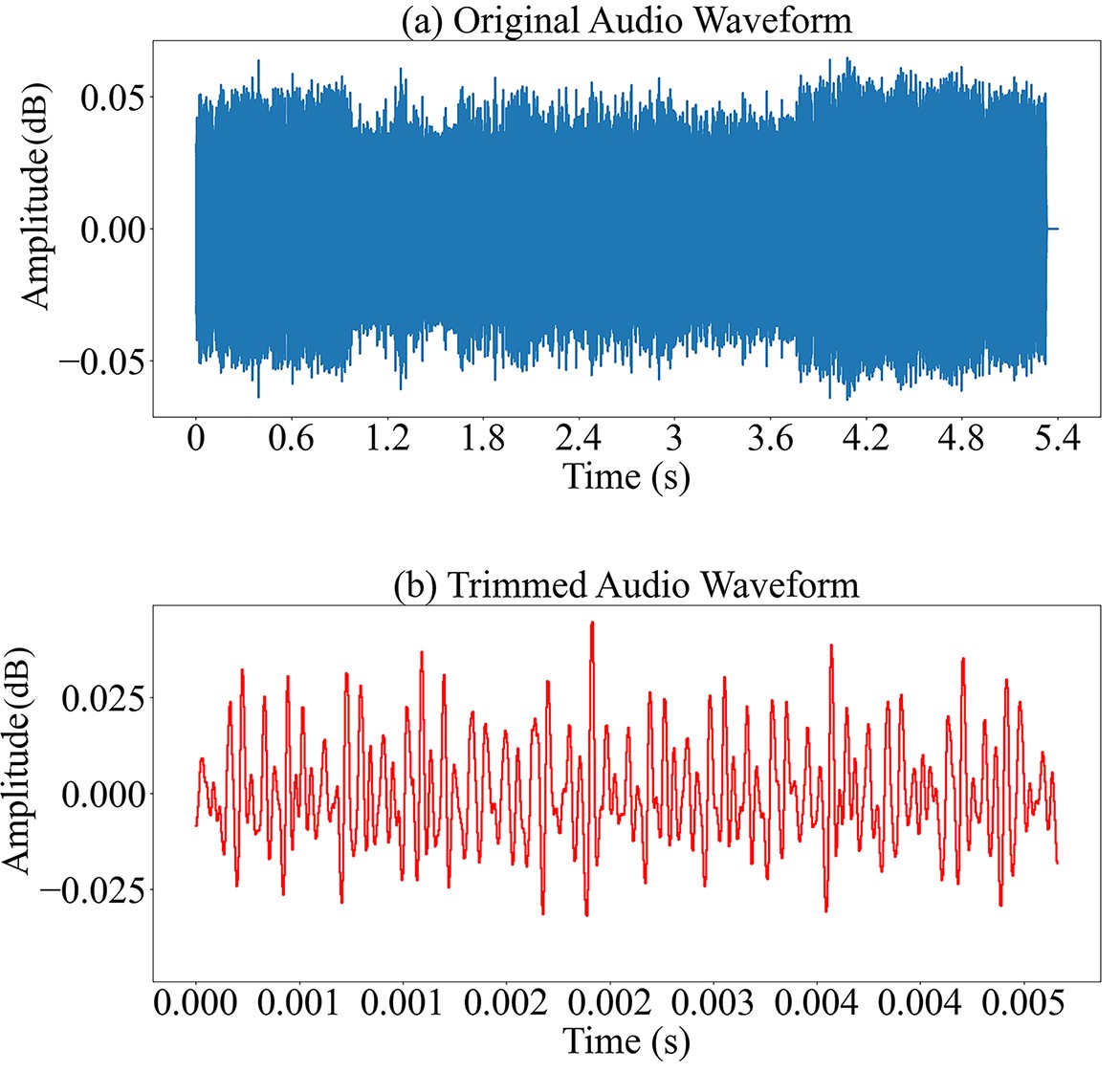
The MFCCs are extracted as the audio features, which are representations of the short-term power spectrum of a sound signal. First of all, all audio signals are collected in.wav format, loaded, and processed with the popular audio processing package “librosa” [35]. In order to increase the alignment of audio signals and reduce redundant information, all data samples are sliced into a uniform duration of 1 s. An example of an original 5.4 s long audio signal and a sliced piece of the same signal is shown in figure 4. After slicing, a first-order high-pass filter is applied to these trimmed samples to boost the higher-frequency content of the signal, which is desired, while attenuating low-frequency noise and disturbances. The high-pass filter follows the below principle:
| y(n) = x(n) - \alpha \cdot x(n-1). | (6) |
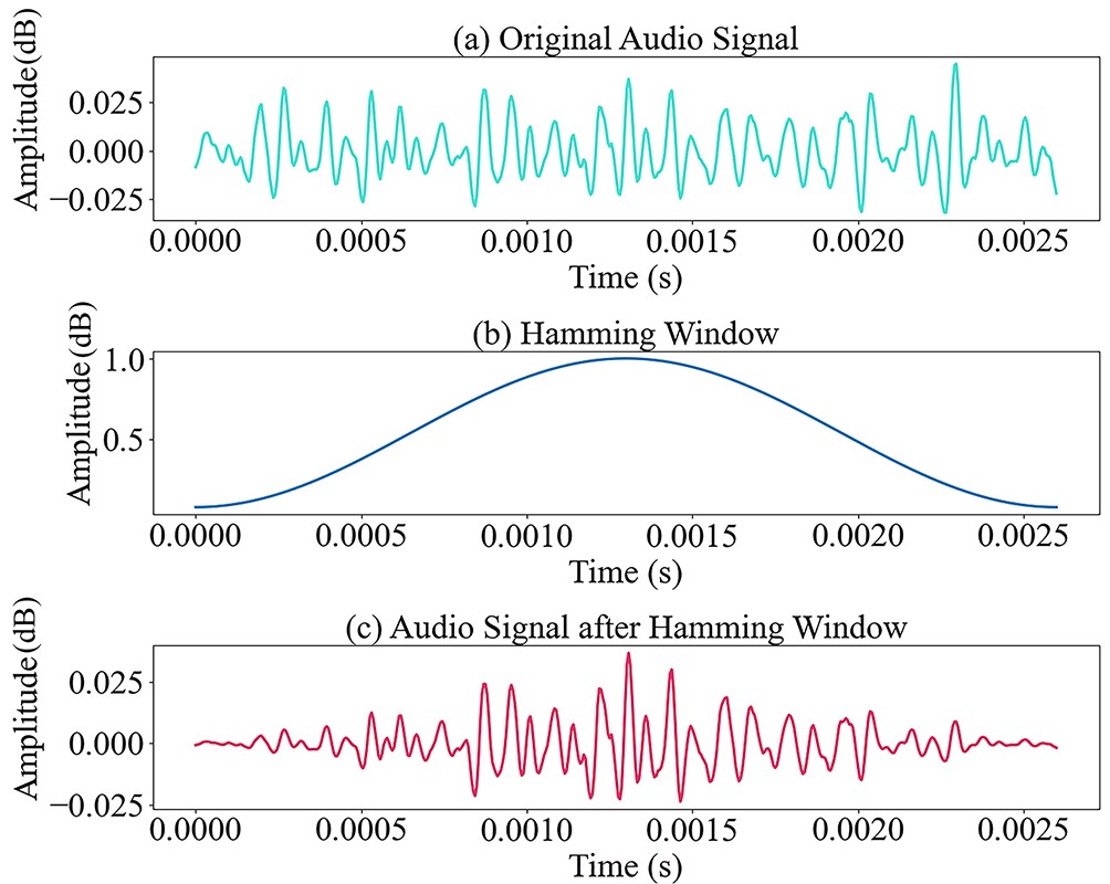
In equation (6), the parameter \alpha is a coefficient in the high-pass filter formula, determining how much of the past signal influences the current output. It helps emphasize the high-frequency components of the signal by attenuating lower frequencies. The filtered audio signal is divided into short overlapping frames to ensure that the characteristics of the signal can be captured accurately over time, as audio signals are not stationary. For the purpose of reducing spectral leakage effects when performing the Fourier transform, each frame of the audio sample is multiplied by a window function (e.g., Hamming window), which can be expressed as:
| W(n) = (1-a) - a \cdot {\rm{cos}}(w \cdot {\text{π}} \cdot n / N),\qquad a\leqslant n \leqslant N. | (7) |
For equation (7), a refers to the amplitude factor of the Hamming window, a function used to reduce signal discontinuities at the edges of a frame in spectral analysis. It shapes the window to minimize spectral leakage during the Fourier transform. The resulting sample from the Hamming window is displayed in figure 5, from which we can see that the original signal is smoothed by the Hamming window by giving more weight to the central part of the segment and less weight to the edges. This is useful in emphasizing the central portion of the signal while reducing the impact of transient or noisy edges, so that the abrupt discontinuities at the edges of the segment are reduced and the spectral leakage is minimized.
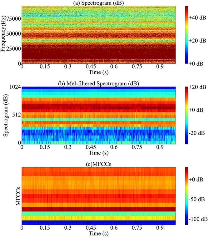
To obtain the spectrogram of the audio sample, the short time fourier transform (STFT) is applied to each frame to convert the signal from the time domain to the frequency domain. Even though the STFT reduces the sample dimension based on the original audio signal, the features derived from the STFT are still high-dimensional and not suitable for machine learning models. Mel filter banks are used to reduce the dimensionality of the frequency domain representation, which transforms the continuous spectrum of frequencies into a set of filter bank energies or coefficients that capture essential spectral characteristics while reducing redundancy. Meanwhile, Mel filter banks emphasize important acoustic features of the audio signal, which are more closely spaced in the Mel domain, making it easier to distinguish them. The logarithm of the filter bank energies is computed, which helps in approximating the logarithmic perception of loudness in human hearing. The relationship between the Mel value and the frequency value is as follows:
| m=2595\rm{\times log}_{10}(1+\mathit{f}/700). | (8) |
Finally, the logarithmic energy output of the filter bank is continuously transformed into a discrete cosine transform (DCT) to obtain MFCCs. Figure 6 shows the transformations of an STFT spectrogram to MFCCs. We can see from this figure that the audio features are reduced from a high dimension after STFT to only 20 MFCCs, which can be fed to our machine learning models as predictors.
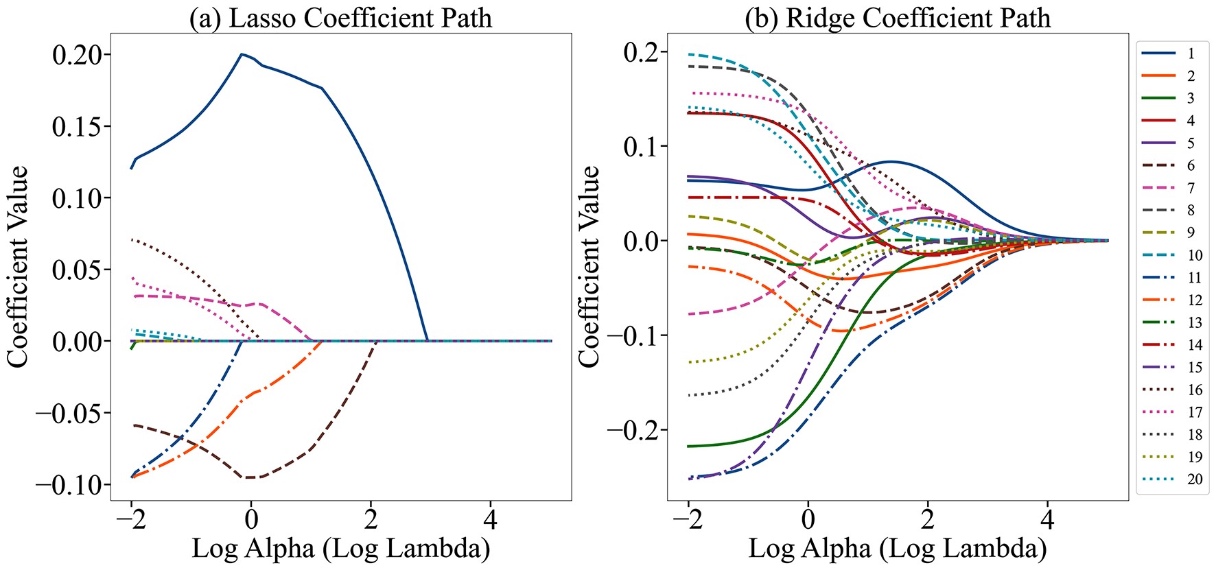
In this study, the entire dataset was first shuffled to increase randomness before being divided into training and test sets, with an 80% to 20% split. In the Linear Regression model, both Lasso and Ridge regularization techniques were applied to optimize the selection of coefficients from the 20 MFCCs. The impact of the regularization penalty, denoted as “alpha”, on the coefficient values during the training phase is depicted in figure 7. This figure illustrates how an increase in the “alpha” value leads to a reduction in the coefficients’ magnitudes to minimize the penalty. Moreover, Lasso regularization has the capability to reduce some coefficients to zero, effectively eliminating certain features, whereas Ridge regularization reduces the magnitude of all coefficients, albeit without completely zeroing any.
The optimal “alpha” value identified through Lasso regularization was 0.01, resulting in a set of coefficients. Several coefficients were reduced to zero, indicating the removal of those features from the model, while the non-zero coefficients highlight the features that remained influential in the model. Conversely, the best “alpha” value for Ridge regularization was determined to be 0.305. The resulting coefficients were all non-zero but some were notably small, indicating a significant reduction in their influence on the model. With the optimal coefficients determined through Lasso and Ridge regularizations, predictions were made on the test datasets for discharge power and distances. The performance of linear regression with Lasso and Ridge regularizations is measured by the MSE and R -squared values and is shown in table 1.
| Model | MSE (power (W)) | MSE (distance (mm)) | R -squared (power (W)) | R -squared (distance (mm)) |
| Linear Regression Lasso | 0.01088 | 0.18935 | 0.88335 | 0.89232 |
| Linear Regression Ridge | 0.01298 | 0.17484 | 0.86091 | 0.90057 |
| kNN | 0.00571 | 0.27913 | 0.93877 | 0.84126 |
| Random Forest | 0.00757 | 0.10186 | 0.91887 | 0.94208 |
 DownLoad:
CSV
DownLoad:
CSV
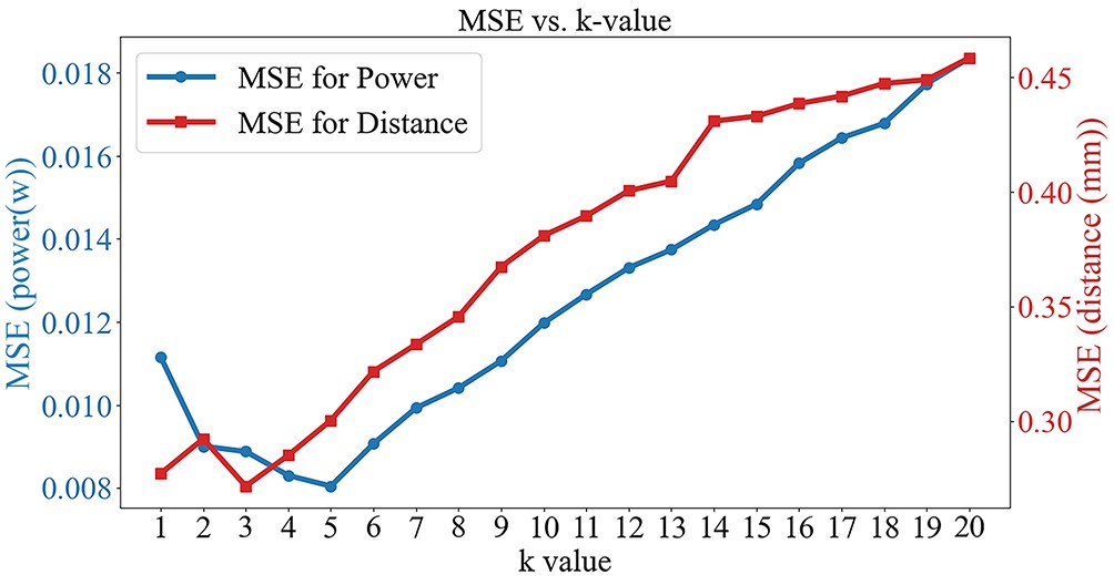
During the building of the kNN model, it is critical to select the optimal number of nearest neighbors, which is denoted as the k-value. The k-value plays a significant role in balancing the model’s bias and variance, directly impacting its predictive performance. To identify the most suitable k-value for accurate predictions, an extensive evaluation was conducted across a spectrum of k-values, ranging from 1 to 20. The outcomes of this evaluation are illustrated in figure 8, which details the MSE associated with each k-value for both power and distance predictions. The analysis revealed that a k-value of 3 yielded the most accurate predictions for discharge power, minimizing the MSE to its lowest point for this particular prediction task. Similarly, for the prediction of discharge distance, a k-value of 5 was identified as optimal, also characterized by the lowest MSE. Based on these findings, a k-value of 3 was adopted for subsequent power prediction tasks within the kNN model framework, while a k-value of 5 was chosen for distance predictions. The predictive efficacy of the kNN model, employing these optimized k-values, was further tested on a separate test dataset. The results of these predictions are presented in table 1.
Unlike Linear Regression and kNN models, which select features through manual settings or regularization techniques, the Random Forest algorithm can achieve feature extraction with its inherent structure. In other words, the Random Forest model does not require the preliminary step of feature selection. The predictions on discharge power and distance made by the Random Forest model, evaluated in terms of MSE and R -squared values, are shown in table 1. Among all three models, the kNN model distinguished itself in the prediction of discharge power, achieving an exceptionally low MSE of 0.005 and an R -squared value of 0.938. This indicates that the kNN model, with its optimized k-value, was particularly adept at capturing the nuances of power prediction, reflecting a high degree of predictive accuracy and an excellent fit to the data. The Random Forest also exhibits good performance in discharge power prediction, with a relatively low MSE (0.00757) and a high R -squared value (0.91887). The predictions of Linear Regression models with both Lasso and Ridge regularizations show less satisfactory results than kNN and Random Forest, which is expected since the Linear Regression model is much simpler. On the other hand, the predictions on discharge distance, for all three models, are less accurate with MSEs ranging from 0.10 to 0.28 due to the discrete input labels of discharge distances. If more experimental data with continuous discharge distances can be fed into our models, the predictions on discharge distance should see a noticeable improvement.
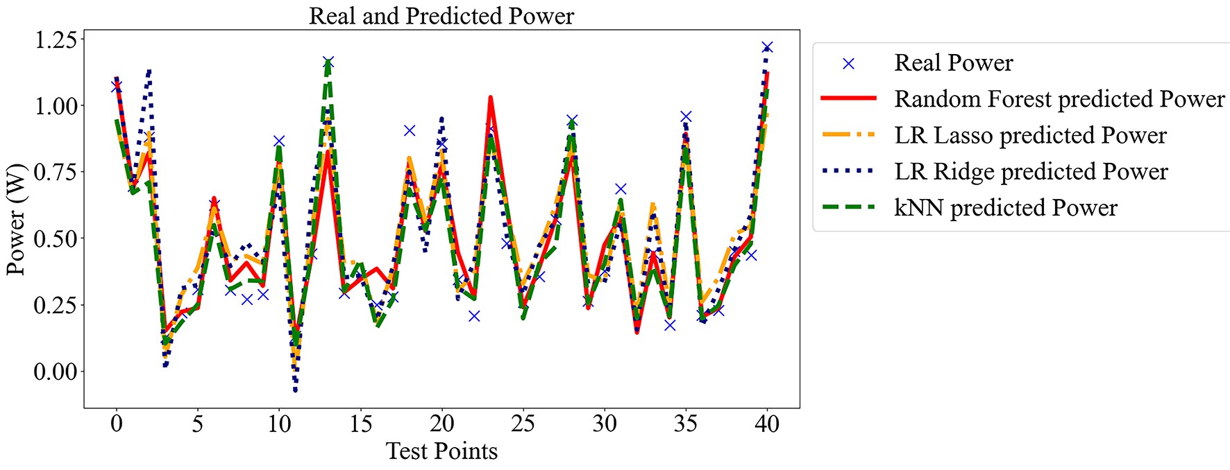
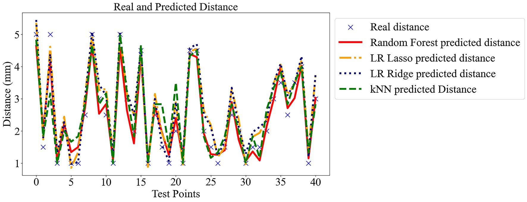
In addition to the evaluation metrics such as MSE and R -squared values detailed in table 1, this study also presents a visual analysis of each model’s predictive performance through the fitting curves depicted in figures 9 and 10. These figures illustrate the models’ predictions for discharge power and distance on 40 test points, providing a graphical representation of the predictive accuracy and the models’ ability to capture the underlying data patterns. The test data points, which were randomized prior to training and testing to ensure a robust model evaluation, are depicted as blue crosses in these figures. The colored lines in both figures stand for the predictive outcomes made by different models on both power output and discharge distance.
From the above figures, we can tell all three models show good prediction and fitting performance, capturing the distribution patterns under real datasets. Specifically, kNN and Random Forest exhibit the best performance by nearly capturing all the test data points in both discharge power and distance. The Linear Regression model, though less accurate, also captures the overall pattern and most of the test data points. The results obtained from figures 9 and 10 are in accordance with the MSE and R -squared values shown in table 1.
The electro-acoustic signals generated by discharges contain rich information about discharge plasma parameters, making them easily accessible and an ideal, non-invasive medium for diagnosing discharge plasma parameters. This study collects electro-acoustic signals produced by a typical spark discharge, along with discharge power and distance data, and utilizes three different machine learning methods (including Linear Regression, kNN, and Random Forest) to enable rapid prediction of discharge power and distance parameters using the sound signals from spark discharges. This study employs MFCCs for feature extraction from the complex raw sound signals, and through the application of first-order high-pass filtering, the Hamming window function, and STFT, it effectively captures the key features of discharge sound signals under various conditions.
The models utilized in the paper demonstrate impressive performance in terms of prediction accuracy and fitting ability, with their predictive R^2 values all exceeding 0.860. Among them, kNN shows the best performance in predicting discharge power, featuring the lowest mean square error (MSE = 0.005) and the highest determination coefficient ( R^2 = 0.938). This research successfully establishes the connection between electro-acoustic signals and the power and discharge gap distance using machine learning techniques, offering novel perspectives and foundational support for the online tracking and instantaneous assessment of plasma characteristics. Additionally, using advanced machine learning and deep learning models is a promising way to improve the prediction of discharge parameters, as these models can uncover complex patterns missed by simpler ones. We also plan to expand our experiments to cover more discharge scenarios for a better understanding of the phenomena. This broader approach not only matches suggested research directions but also paves the way for new applications in environmental science, materials engineering, and bio-medicine.
This work was partially supported by National Natural Science Foundation of China (No. 52377155) and the State Key Laboratory of Reliability and Intelligence of Electrical Equipment (No. EERI-KF2021001), Hebei University of Technology.
| [1] |
Laroussi M et al 2022 IEEE Trans. Radiat. Plasma Med. Sci. 6 127 doi: 10.1109/TRPMS.2021.3135118
|
| [2] |
Lu X et al 2016 Phys. Rep. 630 1 doi: 10.1016/j.physrep.2016.03.003
|
| [3] |
Graves D B et al 2012 J. Phys. D: Appl. Phys. 45 263001 doi: 10.1088/0022-3727/45/26/263001
|
| [4] |
von Woedtke T et al 2013 Phys. Rep. 530 291 doi: 10.1016/j.physrep.2013.05.005
|
| [5] |
Lu X et al 2014 Phys. Rep. 540 123 doi: 10.1016/j.physrep.2014.02.006
|
| [6] |
Snoeckx R et al 2021 Combust. Flame 225 1 doi: 10.1016/j.combustflame.2020.10.028
|
| [7] |
Starikovskiy A et al 2013 Progr. Energy Combust. Sci. 39 61 doi: 10.1016/j.pecs.2012.05.003
|
| [8] |
Matveev I B et al 2010 IEEE Trans. Plasma Sci. 38 3257 doi: 10.1109/TPS.2010.2091153
|
| [9] |
Bogaerts A et al 2022 Plasma Sources Sci. Technol. 31 053002 doi: 10.1088/1361-6595/ac5f8e
|
| [10] |
Corke T C et al 2010 Annu. Rev. Fluid Mechan. 42 505 doi: 10.1146/annurev-fluid-121108-145550
|
| [11] |
Penkov O V et al 2015 J. Coat. Technol. Res. 12 225 doi: 10.1007/s11998-014-9638-z
|
| [12] |
Dingemans G et al 2012 J. Electrochem. Soc. 159 H277 doi: 10.1149/2.067203jes
|
| [13] |
Grosse-Kreul S et al 2015 Plasma Sources Sci. Technol. 24 044008 doi: 10.1088/0963-0252/24/4/044008
|
| [14] |
Pei X et al 2013 Plasma Sources Sci. Technol. 22 025023 doi: 10.1088/0963-0252/22/2/025023
|
| [15] |
Lo A et al 2012 Appl. Phys. B: Lasers Opt. 107 229 doi: 10.1007/s00340-012-4874-3
|
| [16] |
Wu S et al 2022 Plasma Processes Polym 19 e2100164 doi: 10.1002/ppap.202100164
|
| [17] |
Xiong Q et al 2009 J. Appl. Phys. 106 083302 doi: 10.1063/1.3239512
|
| [18] |
Boinet M et al 2004 NDT E Int. 37 213 doi: 10.1016/j.ndteint.2003.09.011
|
| [19] |
Law V J et al 2011 Plasma Sources Sci. Technol. 20 035024 doi: 10.1088/0963-0252/20/3/035024
|
| [20] |
O’Connor N et al 2011 J. Appl. Phys. 110 013308 doi: 10.1063/1.3587225
|
| [21] |
Ghosh P et al 2024 J. Phys. D: Appl. Phys. 57 014001 doi: 10.1088/1361-6463/acfdb6
|
| [22] |
Lin L et al 2023 J. Phys. D: Appl. Phys. 57 015203 doi: 10.1088/1361-6463/acfcc7
|
| [23] |
Zhong L et al 2023 J. Phys. D: Appl. Phys. 56 074006 doi: 10.1088/1361-6463/acb604
|
| [24] |
Sibanyoni H et al 2020 Proc. 21st Int. Symp. High Volt. Eng. 599 1430
|
| [25] |
Shojaei K and Mangolini L 2021 J. Phys. D: Appl. Phys. 54 265202 doi: 10.1088/1361-6463/abf61e
|
| [26] |
Gidon D et al 2019 IEEE Trans. Radiat. Plasma Med. Sci. 3 597 doi: 10.1109/TRPMS.2019.2910220
|
| [27] |
Chang J et al 2023 IEEE Trans. Plasma Sci. 51 311 doi: 10.1109/TPS.2022.3185029
|
| [28] |
Zhang W et al 2022 J. Phys. D: Appl. Phys. 55 26LT01 doi: 10.1088/1361-6463/ac5d04
|
| [29] |
Yakubovich V A et al 2021 Vestnik St. Petersb. Univ. Math. 54 384 doi: 10.1134/S106345412104021X
|
| [30] |
Tsai Y et al 2018 IFAC-PapersOnLine 51 13 doi: 10.1016/j.ifacol.2018.09.237
|
| [31] |
Huang G et al 2006 Neurocomputing 70 489 doi: 10.1016/j.neucom.2005.12.126
|
| [32] |
Noi P T and Kappas M 2018 Sensors 18 18 doi: 10.3390/s18010018
|
| [33] |
Belgiu M et al 2016 ISPRS J. Photogramm. Remote Sens. 114 24 doi: 10.1016/j.isprsjprs.2016.01.011
|
| [34] |
Breiman L et al 2001 Mach. Learn. 45 5 doi: 10.1023/A:1010933404324
|
| [35] |
McFee B et al 2015 librosa: Audio and Music Signal Analysis in Python Proc. 14th Python Sci. Conf. 1 18 doi: 10.25080/majora-7b98e3ed-003
|
Figures(10) / Tables(1)
Supported by: Beijing Renhe Information Technology Co., Ltd. 
| Model | MSE (power (W)) | MSE (distance (mm)) | R -squared (power (W)) | R -squared (distance (mm)) |
| Linear Regression Lasso | 0.01088 | 0.18935 | 0.88335 | 0.89232 |
| Linear Regression Ridge | 0.01298 | 0.17484 | 0.86091 | 0.90057 |
| kNN | 0.00571 | 0.27913 | 0.93877 | 0.84126 |
| Random Forest | 0.00757 | 0.10186 | 0.91887 | 0.94208 |
DownLoad:
CSV