Invariant manifold growth formula in cylindrical coordinates and its application for magnetically confined fusion

1.   Introduction

In the tokamak community, the magnetic topology is, most of the time, assumed to be nested flux surfaces, e.g. in Grad–Shafranov equation, EFIT, VMEC, etc. Based on this assumption, people have established a dedicated theory [1] of magnetic coordinates in which all magnetic field lines on a flux surface are straight. Nevertheless, the three-dimensional (3D) effect is ubiquitous in real-world fusion experiments since any facility in fusion machines, except the central solenoid and poloidal field coils, is 3D. For example, the toroidal field coils exhibit a ripple effect, the microwave and radio-frequency wave heating methods impose their distinctive localized distribution pattern of the induced current, and the neutral beam injection has an obvious non-axisymmetric current effect. Furthermore, most instability modes of plasma, such as the tearing mode and sawtooth mode, imply a significant 3D topology change of the magnetic field. The 3D effect is unavoidable in the magnetically confined fusion research, thereby requiring a deeper comprehension on the global field structure.

An enormous amount of fusion research has attempted to stimulate a chaotic field layer at the plasma boundary by either resonant magnetic perturbation (RMP) coils [2–4] or other means [5] to mitigate destructive type-I edge localized modes (ELMs). The theoretical basis was established in 1983 by Cary and Littlejohn [6] to estimate how wide the island chains are when an axisymmetric magnetic field is perturbed by a non-axisymmetric one, after which hundreds of researchers implement RMP coils to mitigate and suppress ELMs [7, 8]. The method is called magnetic spectrum analysis nowadays, heavily relying on Fourier transform of the radial component of the perturbation field, which is a linear operation in functional spaces. Therefore the utility of magnetic spectrum analysis is limited inside the plasma and becomes less and less accurate as the perturbation is strengthened, because Fourier transform is merely a linear operation and not capable of explaining the nonlinear behaviour.

With the aid of modern dynamical system theory, the structure of a 3D vector field can be comprehended and analyzed in terms of invariant manifolds [9, 10]. Various numerical methods have been developed to grow them [11–16]. Kuznetsov and Meijer systematically investigated the bifurcation behaviour of 1D and 2D maps when their parameters change [17, 18], presenting diverse analytic and numerical methods to study maps. However, the methods taken by mathematicians are too general to capture the essence of a 3D vector field, leaving the analysis as complicated as before.

Since the magnetic field dominates the plasma transport in magnetically confined fusion machines, the evidence of transversely intersecting invariant manifolds shall be easy to observe, which is a signature of chaos. The invariant manifolds are essential to determine the chaotic field regions, which induce a mixing effect inside the plasma. The plasma edge is not suitable to be characterized by a single closed surface when the 3D effect is strong, for which it is proposed to use the notion of invariant manifolds of outmost saddle cycle(s). In fact, it has been observed in some existing simulation [19–22] and experiment results. On EAST, the helical current filaments induced by the lower hybrid wave heating impacted the plasma edge topology and caused an evident splitting of strike points in experiments [5].

If RMP coils are imposed to suppress ELMs in tokamaks, the heat flux pattern at the divertor exhibits a complex toroidally asymmetric distribution, which poses challenges to ITER and DEMO divertor designs [23]. Simulation results demonstrate that the divertor plasma regions with connection to the bulk plasma are dragged further outside when the asymmetry is intensified [24, 25]. The field line connection length and the magnetic footprint (how deep the field lines penetrate into the bulk plasma) distribution at the divertor are usually ribbon-like. The RMP does mitigate or even suppress the ELMs, otherwise which can cause intolerable transient particle and heat flux. On the other hand, significant heat fluxes may arise far from the strike point originally designed for axisymmetric cases [26], possibly damaging the fragile parts of the divertor. Moreover, it remains unknown whether the total heat flux leaked from the bulk plasma is reinforced by the perturbation.

Previous research has attempted to draw the two transversely intersecting manifolds of hyperbolic cycles for 3D toroidal vector fields. Ottino from the community of fluid mechanics [27], Roeder, Rapoport, and Evans from the fusion community [28, 29] have drawn up the relevant figures. Abdullaev has deduced an approximate (to first order in ϵ because Poincaré integral is used) analytic implicit expression of the invariant manifolds of the outmost X-cycle when a single-null configuration is perturbed [30]. This paper carries forward the research and directly deduce the intrinsic analytic formula of the invariant manifolds of hyperbolic cycles without need for approximation.

Section 2 explains the definitions and denotations used in this paper. The theory skeleton of this paper is put in section 3, while the detailed proofs are put in appendix A. Section 4 offers intuitive examples to help understand the theory. Non-Möbiusian/Möbiusian saddle cycles and a dummy X-cycle model are constructed analytically. A real-world numeric example of analyzing a magnetic field timeslice on EAST is presented subsequently. Section 5.1 and appendix B give comparisons with others' works. Section 5.2 is the conclusion.

2.   Definitions and notations

Vector fields are presumed to be at least once continuously differentiable, i.e. of class C¹. Although a vector field is denoted by B, it is worth emphasizing that it does not need to be divergence-free in this paper.

The flow X(x₀, t) induced by the field B and the corresponding flow X_pol(x₀, ϕ_s, ϕ_e) in cylindrical coordinates play a great role in the deduction of theory, especially the latter one (a flow is often denoted by ϕ^t or ϕ(t, x₀) in other literature, but ϕ has been used as the azimuthal angle in this paper). Denotations used are listed in table 1. The symbol $\mathcal{D}$ serves as a differentiation operator w.r.t. the initial condition x₀, as distinguished from those w.r.t. time-like variables t, ϕ_s or ϕ_e.

Table  1.  Denotations.

	Cartesian	Cylindrical
FLT ODE system	$\boldsymbol{\dot x} = {\boldsymbol{B}}(\boldsymbol{x})\overrightarrow {\left\{ {\begin{array}{l} {x = R\cos \phi }\\ {y = R\sin \phi }\\ {z = Z} \end{array}} \right.}$	$\left\{\begin{array}{l}\mathrm{d} x_R / \mathrm{d} x_\phi=R B_R / B_\phi \\ \mathrm{d} x_{Z} / \mathrm{d} x_\phi=R B_Z / B_\phi\end{array}\right.\qquad \qquad (1)$
Init. condition	$\boldsymbol{x}_0=\left(x_{0 x}, x_{0 y}, x_{0 z}\right)$	$\boldsymbol{x}_0=\left(x_{0 R}, x_{0 Z}\right)$
Flow	X(x0, t)	Xpol(x0, ϕs, ϕe), subscripts s for start, e for end
	∂tX(x0, t) = B(X(x0, t))	$\partial_{\phi_{\mathrm{e}}} \boldsymbol{X}_{\mathrm{pol}}\left(\boldsymbol{x}_0, \phi_{\mathrm{s}}, \phi_{\mathrm{e}}\right)=\frac{R \boldsymbol{B}_{\mathrm{pol}}}{B_\phi}\left(\boldsymbol{X}\left(\boldsymbol{x}_0, \phi_{\mathrm{s}}, \phi_{\mathrm{e}}\right)\right.$
Diff w.r.t. x0	${\cal D}\boldsymbol{X}({\boldsymbol{x}_0}, t):{\rm{ }} = \frac{{\partial \boldsymbol{X}({\boldsymbol{x}_0}, t)}}{{\partial ({x_{0x}}, {x_{0y}}, {x_{0z}})}}$	${\cal D}{\boldsymbol{X}_{\mathrm{pol}}}({\boldsymbol{x}_0}, {\phi _{\rm{s}}}, {\phi _{\rm{e}}}):{\rm{ }} = \frac{{\partial {\boldsymbol{X}_{\mathrm{pol}}}({\boldsymbol{x}_0}, {\phi _{\rm{s}}}, {\phi _{\rm{e}}})}}{{\partial ({x_{0R}}, {x_{0Z}})}}$
By chain rule	$\frac{\partial }{{\partial t}}{\cal D}\boldsymbol{X}({\boldsymbol{x}_0}, t) = \nabla \boldsymbol{B}(\boldsymbol{X}({\boldsymbol{x}_0}, t))\;\, {\cal D}\boldsymbol{X}({\boldsymbol{x}_0}, t).\quad \;\;\; (2)$	$\frac{\partial }{{\partial {\phi _{\rm{e}}}}}{\cal D}{\boldsymbol{X}_{\mathrm{pol}}}({\boldsymbol{x}_0}, {\phi _{\rm{s}}}, {\phi _{\rm{e}}}) = \mathbf{A}({\phi _{\rm{e}}})\;\, {\cal D}{\boldsymbol{X}_{\mathrm{pol}}}({\boldsymbol{x}_0}, {\phi _{\rm{s}}}, {\phi _{\rm{e}}}), \;\, \;\, \quad \;\;\; (3)$
		where $\mathbf{A}({\phi _{\rm{e}}}):{\rm{ }} = \frac{{\partial \left({R{\boldsymbol{B}_{\mathrm{pol}}}/{B_\phi }} \right)}}{{\partial (R, Z)}}({\boldsymbol{X}_{\mathrm{pol}}}({\boldsymbol{x}_0}, {\phi _{\rm{s}}}, {\phi _{\rm{e}}}), {\phi _{\rm{e}}})$

 | Show Table

DownLoad: CSV

Naturally, the Poincaré map ${\cal P}({\boldsymbol{x}_0}, \phi )$ with ${\boldsymbol{x}_{\rm{0}}}{\rm{ = }}\left(x_{0 R}, x_{0 Z}\right)$ is defined by the standard R-Z semi-infinite planes Σ(ϕ) at ϕ angles, recording the strike points crossing the planes in one direction. If a trajectory flies around Σ(ϕ) through the opposite semi-infinite plane Σ(ϕ + π), then by definition the Poincaré map does not record the strike point on Σ(ϕ + π). Since the flow X_pol(x₀, ϕ_s, ϕ_e) and the map ${\cal P}({\boldsymbol{x}_0}, \phi )$ are used frequently in this paper, different terminologies are used to distinguish the continuous-time dynamics from the discrete-time one, e.g. equilibrium point, trajectory and cycle are for continuous-time dynamics, while fixed point, orbit and periodic orbit are for discrete-time one.

This paper follows the definitions of stable and unstable manifolds given by Jacob Palis and Welington de Melo [31], (p. 73) for a hyperbolic fixed point (p. 59) and (p. 98) for a hyperbolic cycle (p. 95). In both cases the manifolds are defined by ω- and α-limit sets, so one can unify the manifold definitions in the continuous and discrete dynamics by considering manifolds of a hyperbolic set S (a definition at (p. 160) for the case of a map), since both hyperbolic fixed points and hyperbolic cycles are hyperbolic sets. Note a hyperbolic periodic orbit is also a hyperbolic set, which can be handled by the unified definition. Let (M, f) be a dynamical system, where f is a map ${\cal P}$ or a vector field B defined on a metric space or differentiable manifold M. The stable and unstable manifolds of a hyperbolic invariant set S for f are defined by ω- and α-limit sets, respectively

where the superscripts u and s are short for unstable and stable, respectively. The term hyperbolic ensures the nearby trajectories/orbits on stable (respectively unstable) manifolds approach (respectively get away from) S at an exponential rate, without which the sets defined above are only qualified to be named stable (respectively unstable) sets [32] (p. 257), because the stable manifold theorem [31] (p. 75) requires S to be hyperbolic. Colloquially, the stable (respectively unstable) manifold is the set of points that will flow into (respectively flowed out of) S at an exponential rate [32] (p. 258). Kuznetsov and Meijer simply write f^±k(x) → S as k → ∞ [18] (p. 4), where f is a map, without explaining what they mean by 'converging to a set S', which is suspected to be an alternative denotation of ω- and α-limit sets.

For notational convenience, arguments can be omitted if suitable, e.g. ${\cal D}\boldsymbol{X}(t)$ and ${\cal D}{\boldsymbol{X}_{\rm pol}}({\phi _{\rm{s}}}, {\phi _{\rm{e}}})$ are short for ${\cal D}\boldsymbol{X}({\boldsymbol{x}_0}, {\phi _t})$ and ${\cal D}{\boldsymbol{X}_{\rm pol}}({\boldsymbol{x}_0}, {\phi _{\rm{s}}}, {\phi _{\rm{e}}})$ by omitting x₀, ${\cal D}{{\cal P}^m}(\phi )$ for ${\cal D}{{\cal P}^m}({\boldsymbol{x}_0}, \phi )$, and ${{\cal W}^{{\rm{u}}/{\rm{s}}}}(S)$ for ${{\cal W}^{{\rm{u}}/{\rm{s}}}}(\boldsymbol{f}, S)$.

3.   From field line tracing to invariant manifolds

${\cal D}\boldsymbol{X}$ and ${\cal D}{\boldsymbol{X}_{{\rm{pol}}}}$ imply the change of differential volume and area during FLT, respectively. Suppose a 2D map is written as (x, y) ↦ (u, v). The differential area expands, shrinks, or keeps constant after being mapped, as revealed by the following exterior product of differential 1-forms

As X_pol(ϕ_s, ϕ_e) is a typical 2D map from the section Σ(ϕ_s) to Σ(ϕ_e), the determinant of ${\cal D}{\boldsymbol{X}_{{\rm{pol}}}}({\phi _{\rm{s}}}, {\phi _{\rm{e}}})$, denoted by $\left| {{\cal D}{\boldsymbol{X}_{\mathrm{pol}}}({\phi _{\rm{s}}}, {\phi _{\rm{e}}})} \right|$, is indeed the same thing as ∂_xu ∂_yv − ∂_yu ∂_xv. One could be curious about the geometric meaning of $\left| {{\cal D}{\boldsymbol{X}_{{\rm{pol}}}}({\phi _{\rm{s}}}, {\phi _{\rm{e}}})} \right|$ and conjecture that it must be related to the divergence of the field, since it has been well-known [33] (p. 408) that for $\left| {{\cal D}\boldsymbol{X}({\boldsymbol{x}_0}, t)} \right|$

which indicates that, for a divergence-free field, $\left| {{\cal D}\boldsymbol{X}({\boldsymbol{x}_0}, t)} \right|$ is always zero. A similar formula for $\left| {{\cal D}{\boldsymbol{X}_{{\rm{pol}}}}({\phi _{\rm{s}}}, {\phi _{\rm{e}}})} \right|$ is deduced (proof in appendix A.1) to reveal the relationship between $\left| {{\cal D}{\boldsymbol{X}_{{\rm{pol}}}}({\phi _{\rm{s}}}, {\phi _{\rm{e}}})} \right|$ and the divergence along the corresponding trajectory X_pol(ϕ_s, ϕ), ϕ_s ≤ ϕ ≤ ϕ_e, as shown below

which applies to 3D vector fields of class C¹, no matter whether they are divergence-free or not.

More importantly, ${\cal D}{{\cal P}^{ \pm m}}({\boldsymbol{x}_0}, \phi )$ with x₀ on an X-cycle γ of m toroidal turn(s) decides the two X-leg directions of the X-point. ${\cal D}{{\cal P}^m}({\boldsymbol{x}_0}, \phi ) = {\cal D}{\boldsymbol{X}_{\mathrm{pol}}}({\boldsymbol{x}_0}, \phi , \phi + 2m\pi )$ if B_ϕ is positive everywhere. It is the two eigenvectors of ${\cal D}{{\cal P}^m}({\boldsymbol{x}_0}, \phi )$ that dictate towards which direction the two invariant manifolds of that hyperbolic cycle grow at the beginning. However, ${\cal D}{{\cal P}^m}({\boldsymbol{x}_0}, \phi )$ itself is more difficult to solve for than its determinant, which is a constant independent of ϕ for the cycle. This is because the right-hand side of equation (8) becomes a constant as ϕ_e = ϕ_s + 2mπ, i.e.

Unlike the determinant $\left| {{\cal D}{{\cal P}^{ \pm m}}({\boldsymbol{x}_0}, \phi )} \right|$, the matrix ${\cal D}{{\cal P}^{ \pm m}}({\boldsymbol{x}_0}, \phi )$ varies w.r.t the azimuthal angle ϕ. The evolution rule of ${\cal D}{{\cal P}^{ \pm m}}({\boldsymbol{x}_0}, \phi )$ w.r.t. ϕ is revealed in section 3.1.

To calculate ${\cal D}{\boldsymbol{X}_{{\rm{pol}}}}({\phi _{\rm{s}}}, {\phi _{\rm{e}}})$ by integrating equation (3) requires that B_ϕ on the trajectory does not change its sign. Otherwise, RB_pol/B_ϕ would be undefined due to zero B_ϕ. These trajectories are not useless and could be well-defined in Cartesian coordinates. Suppose a trajectory goes from ϕ_s to ϕ_e, during which B_ϕ may change its sign for several times. The zero B_ϕ singularities cause inconvenience to solving for the ${\cal D}{\boldsymbol{X}_{{\rm{pol}}}}({\phi _{\rm{s}}}, {\phi _{\rm{e}}})$. To get around the zero B_ϕ singularity issue, one can solve for the corresponding ${\cal D}\boldsymbol{X}$ first and then change its coordinates back to the cylindrical system. The following ${\cal D}\boldsymbol{X}$ to ${\cal D}{\boldsymbol{X}_{{\rm{pol}}}}$ formula (proof in appendix A.2) tells how to do so

where the subscripts start and end mean that the corresponding matrices are evaluated at the starting and ending point of this trajectory, respectively, i.e. $\left(\boldsymbol{X}_{\mathrm{pol}}\left(\phi_{\mathrm{s}}, \phi_{\mathrm{s}}\right), \phi_{\mathrm{s}}\right)$ and $\left(\boldsymbol{X}_{\mathrm{pol}}\left(\phi_{\mathrm{s}}, \phi_{\mathrm{e}}\right), \phi_{\mathrm{e}}\right)$.

3.1   The evolution of ${\cal D}{{\cal P}^{ \pm m}}$ along a cycle

For a cycle of m toroidal turn(s), the relationship among the ${\cal D}{{\cal P}^{ \pm m}}(\phi )$ matrices at neighboring sections is desired, without which the calculation of their eigenvectors would spend unnecessarily enormous computational resources. The most primitive approach is definitely repeating the integration of equation (3) from ϕ_s to ϕ_s + 2mπ once and once again for various ϕ_s, i.e. from ϕ₁ to ϕ₁ + 2mπ, from ϕ₂ to ϕ₂ + 2mπ... To avoid this horribly primitive approach, the following ${\cal D}{{\cal P}^{ \pm m}}$ evolution formula is deduced (proof in appendix A.3) to reveal how ${\cal D}{{\cal P}^{ \pm m}}(\phi )$ varies along the cycle

where the square bracket denotes the commutator, i.e. $[\mathbf{A}, \mathbf{B}]=\mathbf{A} \mathbf{B}-\mathbf{B} \mathbf{A}$. In the dummy X-cycle demonstration figures 2(a) and (b), section 4.2, arrows are drawn to indicate the directions of eigenvectors.

The ${\cal D}{{\cal P}^{ \pm m}}$ evolution formula can be applied to cycles in autonomous n-dimensional flows (n ≥ 2 and finite). For other dimensions than n = 3, the denotation $\left| {{\cal D}\boldsymbol{X}({\boldsymbol{x}_0}, T)} \right|$ is preferred than $\left| {{\cal D}{{\cal P}^m}(\phi )} \right|$, where T is the period of the cycle, because the former one does not rely on the choice of Poincaré section. The n-dimensional version of equation (11) in Cartesian coordinates is shown below

Furthermore, it is desirable to deduce how an eigenvector of ${\cal D}{{\cal P}^{ \pm m}}(\phi )$ evolves along an X-cycle, so that one can get rid of the arbitrariness of the computed eigenvector direction, which depends on the specific eigen-decomposition numeric algorithm. If the eigenvector rotates a lot during evolution, the employed numerical method might give a reversed direction without consistency, i.e. the computed eigenvector may jump to the opposite side suddenly. The following ${\cal D}{{\cal P}^{ \pm m}}$ eigenvector evolution formula (proof in appendix A.4) extracts the underlying rule governing the rotation of ${\cal D}{{\cal P}^m}(\phi )$ eigenvectors along the cycle. Let the eigenvectors of ${\cal D}{{\cal P}^{ \pm m}}(\phi )$ be denoted by $\boldsymbol{v}_i=\left[\cos \theta_i(\phi), \sin \theta_i(\phi)\right]^{\mathrm{T}}, i \in\{1, 2\}$. The derivative of Θ(ϕ) : = diag(θ₁, θ₂) w.r.t. ϕ satisfies

where V : = [v₁, v₂] and Λ : = diag(λ₁, λ₂). We discovered in numeric implementation that the formula above (13), though accurate, but encounters some numeric issue while handling the X-cycles in island chains, because the two eigenvectors are so close to each other that some matrices in this formula might become pretty singular, i.e. have big conditional number. A much more robust way is to directly use ${\cal D}{{\cal P}^m}(\phi )$ evolution formula (11) to evolve ${\cal D}{{\cal P}^m}(\phi )$ and later comb the directions of eigenvectors.

Traditionally, fixed points of 2D maps are classified into hyperbolic, elliptic, and parabolic types based on their Jacobian eigenvalues. For the cycles of 3D flows, the authors want to imitate this naming convention. It is worth emphasizing that the eigenvalues of ${\cal D}{{\cal P}^{ \pm m}}(\phi )$ keep constant during evolution.⁴ Hence, it is safe to classify a cycle γ of m toroidal turn (s) by its ${\cal D}{{\cal P}^m}$ eigenvalues. The λ-invariance ensures the safety of such classification, because one does not need to worry about that the ${\cal D}{{\cal P}^m}(\phi )$ eigenvalues at different ϕ are different.

⁴ This is a well-known fact in the ODE community, because it is easy to verify that ${\cal D}{\cal P}({\phi _2})$ and ${\cal D}{\cal P}({\phi _1})$ are similar by checking ${\cal D}{\cal P}({\phi _2}) = {\cal D}{\boldsymbol{X}_{{\rm{pol}}}}{({\phi _2}, {\phi _1})^{ - 1}}\;\, {\cal D}{\cal P}({\phi _1})\;\, {\cal D}{\boldsymbol{X}_{{\rm{pol}}}}({\phi _2}, {\phi _1})$. The commutator form of the right-hand side of the evolution formulas (11) and (12) also ensures the λ-invariance. Let x_i be a right eigenvector of ${\cal D}{{\cal P}^{ \pm m}}$ and $\mathit{\boldsymbol{y}}_i^T$ the corresponding left eigenvector

Given a univariate matrix function A(ϕ), the derivative of its eigenvalue w.r.t. the single parameter ϕ satisfies $\lambda_i^{\prime}=\boldsymbol{y}_i^{\mathrm{T}} \mathbf{A}^{\prime} \boldsymbol{x}_i$ [34]. Now substitute A by ${\cal D}{{\cal P}^{ \pm m}}$ as shown below. It immediately lets us know both λ_i(ϕ) of ${\cal D}{{\cal P}^{ \pm m}}(\phi )$ do not change with ϕ

If both eigenvalues of ${\cal D}{{\cal P}^m}$ are not on the unit circle $\mathbb{S}$ of $\mathbb{C}$, the cycle is said to be hyperbolic.⁵ If only one eigenvalue on the unit circle, the cycle is called partially hyperbolic (but not fully hyperbolic). If both eigenvalues are on $\mathbb{S}$ but neither equal 1 nor −1, the cycle is defined to be elliptic. If the two eigenvalues are identical to 1 or −1, the cycle is defined to be parabolic.

⁵ This definition is equivalent to the conventional one in [31] (p. 95), whose Poincaré section is chosen to be transversal to the local vector field.

Furthermore, a saddle cycle is defined to be one with |λ₁| < 1, |λ₂| > 1. Those saddle cycles with both eigenvalues negative (respectively positive) are called Möbiusian (respectively non-Möbiusian). Note that the Möbiusian cycle defined here is different from the classical Möbiusian strip. The cycles with both λ inside (respectively outside) the unit circle $\mathbb{S}$ of $\mathbb{C}$ are defined to be sinking (respectively sourcing) cycles

Magnetic fields are typical divergence-free fields, in which the so-called X-cycles, O-cycles, and the cycles on rational flux surfaces can now be formally defined as hyperbolic (meanwhile saddle), elliptic, and parabolic, respectively.

3.2   Invariant manifold growth formula in cylindrical coordinates

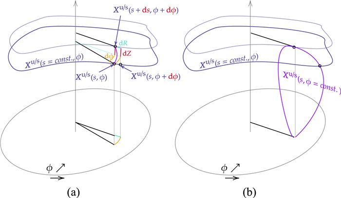
Let γ be a hyperbolic cycle with real eigenvalues of ${\cal D}{{\cal P}^m}$. Since the invariant manifold of γ may grow endlessly, one of the two parameters of the manifold is naturally chosen to be the arc length s of the curves intersected by the 2D manifold ${{\cal W}^{{\rm{u}}/{\rm{s}}}}(\boldsymbol{B}, \gamma )$ and R-Z cross-sections. For the other coordinate, the azimuthal angle ϕ is chosen. Define that s = 0 on the cycle and s increases towards the positive infinity as the manifold grows away from the cycle. The diagram (figure A1) in appendix A.5 could be helpful for readers to understand the geometry, which illustrates the relationship among the differentials used. The diagram is put in appendix because those readers who follow the proof there would need it more.

To be accurate, this paper defines a stable/unstable (manifold) branch to be a connected component of the manifold minus its invariant set, i.e. a connected component of ${{\cal W}^{{\rm{u}}/{\rm{s}}}}(\boldsymbol{f}, S)\backslash S$. For example, a saddle fixed point of a 2D map has 2 eigenvectors and 4 invariant branches.

An invariant branch of γ is parameterized to be X^u/s(s, ϕ) = $\left(\boldsymbol{X}_R^{\mathrm{u} / \mathrm{s}}(s, \phi), \boldsymbol{X}_Z^{\mathrm{u} / \mathrm{s}}(s, \phi)\right)$. To deduce the governing equation of X^u/s(s, ϕ), one simply needs to analyse the differential relationship appearing in FLT, which is concluded in the following invariant manifold growth formula (proof in appendix A.5, requiring no more than knowledge of multivariable calculus)

with the initial condition $\left.\partial_s \boldsymbol{X}^{\mathrm{u} / \mathrm{s}}(s, \phi)\right|_{s=0}$ set to be the normalized eigenvector of ${\cal D}{{\cal P}^m}(\phi )$. Naturally, ∂_sX^u/s(s, ϕ) is 2mπ-periodic in ϕ for a non-Möbiusian saddle cycle. The denominator is essentially ds/dϕ, so the sign ± shall take + if the field line moves away from the cycle as ϕ increases. Otherwise, it takes −.

For Möbiusian saddle cycles, the invariant manifolds can be grown similarly with some subtle difference. A non-Möbiusian saddle cycle has two invariant branches for each stable and unstable manifold. But for a Möbiusian saddle cycle, the 'two' branches of a (un)stable manifold are considered as a whole (since they are connected, they are indeed one branch by definition). To parameterize such a branch, double the period of X^u/s(s, ϕ) in ϕ from 2mπ to 4mπ. X^u/s(s, ϕ) is opposite X^u/s(s, ϕ + 2mπ) across the cycle γ. Then the growth formula works again.

The growth formula would not grow a rational⁶ flux surface from aparabolic cycle on that surface, since any field line does not cover that surface. To grow this surface, the ${\cal D}{{\cal P}^{ \pm m}}$ evolution formula is sufficient. One simply needs to move the cycle in the directions of the ${\cal D}{{\cal P}^m}$ eigenvectors step by step. The role of ${\cal D}{{\cal P}^{ \pm m}}$ evolution formula is to accelerate the computation of ${\cal D}{{\cal P}^m}(\phi )$ at all sections. For an irrational flux surface, one can choose a non-invariant 'cycle' which does not obey the FLT ODE system (1) and then employ the growth formula. For example, in an axisymmetric field, pick a 'cycle' whose R, Z coordinates are constants. The growth formula then degenerates into

⁶ In KAM theory, if there exists a diffeomorphism $\varphi :{{\cal T}^d} \to {^d}$ (${^d}$ is the standard d-torus) such that the resulting motion on $\mathbb{T}^d$ is uniform linear but not static, i.e. $\mathrm{d} \boldsymbol{\varphi}(\boldsymbol{x}) / \mathrm{d} t=\boldsymbol{\omega} \in \mathbb{R}^d \backslash\{\mathit{\pmb{0}}\}$ is called a frequency vector (a.k.a. rotation vector) of ${{\cal T}^d}$. A frequency vector ω is said to be rationally dependent or commensurable if there exists a vector $\boldsymbol{k} \in \mathbb{Z}^d \backslash\{\mathit{\pmb{0}}\}$ such that k · ω = 0. Specifically when d = 2, this paper defines ${{\cal T}^2}$ to be a rational (respectively irrational) flux surface if the corresponding ω is commensurable (respectively incommensurable). The frequency vector ω is unique up to a transform of multiplying a square integer matrix A with $\operatorname{det} \mathbf{A}= \pm 1$ (a.k.a. unimodular matrix) [35, 36], i.e. any two frequency vectors ω₁ and ω₂ can be transformed to each other by such a matrix ω₂ = Aω₁. Note that the transform of A does not change the commensurability of ω.

therefore, ∂X^u/s/∂s is parallel to B_pol and of unit length.

If what is known is limited to one section Σ(ϕ) (so ϕ is omitted in this paragraph), then the 2D invariant manifold growth formula degrades to a delay ODE describing 1D invariant manifolds for a 2D map. Let $\left(\boldsymbol{x}_i\right)_{i=1}^m$ be a hyperbolic periodic orbit under ${\cal P}$. Parameterize an 1D invariant branch of ${{\cal W}^{{\rm{u}}/{\rm{s}}}}({{\cal P}^m}, {\boldsymbol{x}_i})$ by its arc length s as ${\mathit{\boldsymbol{X}}^{{\rm{u}}/{\rm{s}}}}(s):{\mathbb{R}_{ \ge 0}} \to {{\mathbb{R}}^2}$, whose inverse is denoted by s(X). Then one can acquire the following equations to grow the manifold by simple analysis along the branch:

where the ellipsis dots … in the denominators, which serve to normalize, denote the same thing as the numerators. Both equations above also hold for an invariant circle C. The only thing that needs to be modified is that the circle should be parameterized as a function $\boldsymbol{X}(s):\mathbb{R} \to C \subset {\mathbb{R}^2}$ of period the circumference of the circle, whose inverse $s(\boldsymbol{X}):C \to \mathbb{R}$ is now a multivalued function.

4.   Demonstration of cycles and invariant manifolds

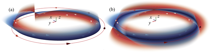
Having developed the systematic theory to characterize the invariant manifolds in 3D autonomous flows, the formulas have been implemented to present readers with a vivid picture. Two analytic and one real-world examples are presented in this section. As the simplest case, the first analytic model is a saddle cycle as shown in figure 1, which can be either non-Möbiusian or Möbiusian. Next is the more complicated dummy X-cycle model as shown in figure 2, which is acquired by twisting the cycle of the first model, i.e. let the R, Z coordinates of the cycle rely on ϕ, instead of being constants. In these two analytic examples, we exhibit the technique to construct a field by the expected trajectories. At last, a timeslice of the magnetic field on EAST is taken as a real-world example as shown in figures 3 and 5, with RMP as the non-axisymmetric perturbation.

Figure  1.  (a) and (b) show the same Möbiusian saddle cycle, of which the field is constructed by equation (26) with parameters: $\left(R_0, Z_0\right)=(1.0, 0.0)$, B_ϕ0 = 2.5, θ_u(ϕ) = ϕ/2 + π/2, θ_s(ϕ) = ϕ/2, λ_u/s = −e^±1/3. The sprouts of two invariant branches are plotted (red for ${{\cal W}^{\rm{u}}}$, blue for ${{\cal W}^{\rm{s}}}$). (a) and (b) draw the manifolds on ϕ ∈ [0, 2π] and [0, 4π] for a half and full poloidal turn, respectively. A trajectory on the unstable branch is drawn for three toroidal turns, i.e. $\phi \in[0, 6 \pi]$.

DownLoad: Full-Size Img PowerPoint

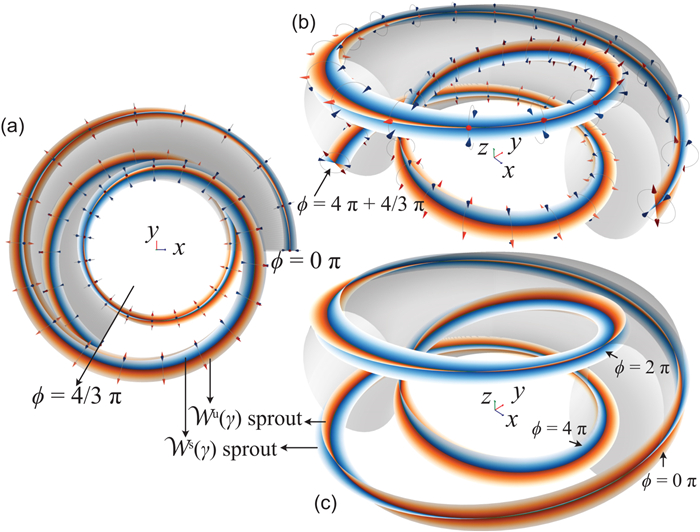
Figure  2.  (a), (b) and (c) show the same dummy X-cycle, of which the field is constructed by equation (32) with parameters: $\left(R_{\mathrm{ax}}, Z_{\mathrm{ax}}\right)=(1.0, 0.0)$, B_{ϕ, ax} = 2.5, ι = n/m = 1/3, $\left(R_{\mathrm{ell}}, Z_{\mathrm{ell}}\right)=(0.3, 0.5)$, θ_u/s(ϕ) = ι ϕ + θ₀ = ϕ/3 + π/2 ± π/9, λ_u/s = e^±1/5. (a) shows it from the top view, (b) and (c) show it from the other view. (a) and (b) draw arrows for the two eigenvectors of ${\cal D}{{\cal P}^3}(\phi )$ and their opposite (blue for λ < 1, red for λ > 1), which is acquired by ${\cal D}{{\cal P}^{ \pm m}}$ evolution formula and shall be consistent with θ_u/s as designed. The sprouts of four invariant branches are plotted (orange for ${{\cal W}^{\rm{u}}}$, blue for ${{\cal W}^{\rm{s}}}$). In (a) and (b), the manifolds are not shown on $\phi \in[6 \pi-2 / 3 \pi, 6 \pi)$, in order not to shelter the eigenvector arrows. A transparent torus with the corresponding elliptic section is drawn for reference.

DownLoad: Full-Size Img PowerPoint

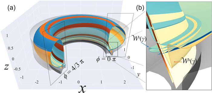
Figure  3.  (a) 3D visualization of the invariant manifolds of the lower X-cycle γ of EAST shot #103950 at 3500 ms (EFIT + vacuum RMP). The first wall is drawn as a transparent grey surface, with the top removed in order not to shelter the manifolds. (b) Enlarged view of (a) at ϕ = 0 near the lower X-point.

DownLoad: Full-Size Img PowerPoint

Figure  4.  Illustration of the numeric algorithm to grow an invariant branch from an X-point for a map.

DownLoad: Full-Size Img PowerPoint

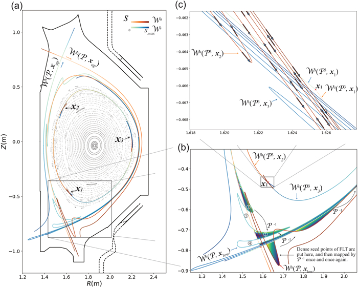
Figure  5.  (a) Poincaré plot at ϕ = 0 of EAST shot #103950 at 3500 ms (EFIT + vacuum RMP). Some invariant manifolds are grown and plotted. (b) Enlarged view of (a) near the lower X-point. Dense scatter points with color are presented to show how the regions are connected by field lines. (c) Enlarged view of (b) near x₁. The blue arrows are drawn according to equation (35).

DownLoad: Full-Size Img PowerPoint

4.1   Non-Möbiusian/Möbiusian saddle cycles

In this section, a saddle cycle model is constructed as an analytic example. Let B_ϕ: = R₀B_ϕ0/R to simulate a tokamak, where B_ϕ0 denotes the toroidal field magnitude at the axis R₀. Suppose B_ϕ is positive. The trajectories on the invariant manifolds of a Möbiusian cycle are expected to be like

where λ_u, λ_s (independent of ϕ) denote the two eigenvalues of ${\cal D}{{\cal P}^m}$, θ_u(ϕ), θ_s(ϕ) denote the corresponding two eigenvectors. If both θ_u and θ_s satisfy θ(ϕ + 2π) = θ(ϕ) + (2k + 1)π, $k \in \mathbb{Z}$, then the cycle is Möbiusian; if they satisfy θ(ϕ + 2π) = θ(ϕ) + 2kπ, $k \in \mathbb{Z}$, then the cycle is non-Möbiusian.

Let $\Delta \boldsymbol{X}_{\mathrm{pol}}(\phi):=\boldsymbol{X}_{\mathrm{pol}}(\phi)-\left[R_0, Z_0\right]^{\mathrm{T}}$. For the unstable trajectories, $\Delta \boldsymbol{X}_{\mathrm{pol}}^{\prime}(\phi)$ is

It is similar for stable trajectories, with λ_u, θ_u(ϕ) replaced by λ_s, θ_s(ϕ). Recall the FLT equation (1) in cylindrical coordinates is $\Delta \boldsymbol{X}_{\mathrm{pol}}^{\prime}(\phi)=R \boldsymbol{B}_{\mathrm{pol}} / \boldsymbol{B}_\phi\left(\boldsymbol{X}_{\mathrm{pol}}(\phi), \phi\right)$. Expand RB_pol/B_ϕ around the cycle

where the subscript c is short for cycle. The FLT equation turns out to be ${\rm{\Delta }}\boldsymbol{X}_{{\rm{pol}}}^\prime (\phi ) = \frac{{\partial R{B_{{\rm{pol}}}}/{B_\phi }}}{{\partial (R, Z)}}\;\, {\rm{\Delta }}{\boldsymbol{X}_{{\rm{pol}}}}(\phi ) + {\cal O}(|{\rm{\Delta }}{\boldsymbol{X}_{{\rm{pol}}}}{|^2})$. To construct a field such that the nearby trajectories are repelled (respectively attracted) at θ_u (respectively θ_s) as expected in equation (19), it is required that

Eigen decomposition is employed to make it possible to let the first orders of the equations above equal at θ_u and θ_s, respectively. As the cost of such decomposition, $\theta_{\mathrm{u}}^{\prime}$ and $\theta_{\mathrm{s}}^{\prime}$ have to be equal, denoted by $\theta^{\prime}$ afterwards.

For the left-hand side of equation (22)

B_ϕ has been defined to be R₀B_ϕ0/R to simulate a tokamak, so ∂_RB_ϕ = −B_ϕ/R. Therefore, the equation above is simplified to

The trajectory equation (19) have been preset by known λ_u, λ_s, θ_u(ϕ), θ_s(ϕ), which means the right-hand side of equation (22) is what we can control. Based on that, the left-hand side of equation (22) can be calculated, i.e. the field we want to construct, after which the linearized B_R, B_Z field is acquired (note B_R, B_Z at the axis have been preset to zero)

The construction is finished. An example of Möbiusian saddle cycle is shown in figure 1.

The non-Möbiusian case is not shown, because it is easy enough to imagine. Some readers may wonder the higher order terms $\frac{\partial^k \boldsymbol{B}_{\mathrm{pol}}}{\partial(R, Z)^k}$, k ≥ 2, which are determined by $\frac{\partial^k R \boldsymbol{B}_{\mathrm{pol}} / B_\phi}{\partial(R, Z)^k}=\mathbf{0}$ in the left-hand side of equation (21).

4.2   Dummy X-cycle

In this subsection, R₀, Z₀ in the last model are replaced (see the trajectory equation (19)) with R_c(ϕ), Z_c(ϕ), two functions dependent on ϕ, respectively. Here, an example expression of R_c(ϕ), Z_c(ϕ) is given

where the subscript c is short for cycle, ell for elliptic, and ax for axis. Similar to the first model, set B_ϕ(R, Z, ϕ) = B_ϕ(R) = R_axB_{ϕ, ax}/R to simulate a tokamak.

The zeroth order components of field expansion are denoted by B_Rc, B_Zc, B_ϕc, to highlight that they are evaluated on the cycle, e.g. B_ϕc = B_ϕ(R_c(ϕ), Z_c(ϕ), ϕ). According to the spiral cycle equation defined above, the following equalities hold

The first order of expansion, ∂B_pol/∂(R, Z), is calculated by equation (25)

Expand the poloidal field around the cycle up to first order,

The construction is finished. A dummy non-Möbiusian X-cycle with q = m/n = 3/1 is shown in figure 2.

4.3   A real-world example

The equilibrium field of EAST shot # 103950 at 3500 ms given by EFIT is taken as background, superimposed with a non-axisymmetric field induced by the RMP coils running in n = 1 mode. The plasma response is not considered here for simplicity. B_ϕ of this shot is negative everywhere, and B_pol at R-Z cross-sections is clockwise.

On locating the periodic points of the Poincaré map, the simplest discrete Newton method ${\boldsymbol{x}_{j + 1}} = {\boldsymbol{x}_j} - h{\left[{{\cal D}\boldsymbol{G}\left({{\boldsymbol{x}_j}} \right)} \right]^{ - 1}}\boldsymbol{G}\left({{\boldsymbol{x}_j}} \right)$ is employed [37], where G(x) : = F(x) − I and I is the identity map. To locate m-periodic orbits of the Poincaré map ${\cal P}(\phi )$ at the section ϕ, our map F is chosen to be the mth iterate of ${\cal P}(\phi )$, that is ${{\cal P}^m}(\phi )$.

After locating the cycle, one needs to know the ${\cal D}{{\cal P}^m}(\phi )$ of this cycle at every section, which is the job of ${\cal D}{{\cal P}^{ \pm m}}$ evolution formula. This formula is a traditional matrix ODE system. The Python function scipy.integrate.solve_ivp and the Julia package DifferentialEquations.jl have prepared a lot of numeric algorithms for such ODEs. Next is to eigen decompose ${\cal D}{{\cal P}^m}(\phi )$, which can be done by, for example, the Python function scipy.linalg.eig. The two eigenvectors of ${\cal D}{{\cal P}^m}(\phi )$ and their opposite are the directions towards which the invariant manifolds grow at the beginning.

Recall the invariant manifold growth formula

only requires two variables on the right-hand side, RB_pol/B_ϕ and ∂X^u/s/∂ϕ. In the numeric implementation, RB_pol/B_ϕ is linearly interpolated on a regular grid of shape $\left[n_R, n_Z, n_\phi\right]$. For ∂X^u/s/∂ϕ, different people have different ways to handle it numerically. In the following two subsections, two approaches to grow manifolds are exhibited.

4.3.1   Naive field line tracing

The simpler scheme is to distribute a line of Poincaré seed points along the eigenvector of a periodic point. To compute the arc length s of a branch of $\mathcal{W}^{\mathrm{u} / \mathrm{s}}\left(\mathcal{P}^m, \boldsymbol{x}_0\right)$ requires the FLT Poincaré orbits used to construct the manifold be ordered, which is achieved with the assistance of the ${\cal D}{{\cal P}^m}(\phi )$ eigenvalues in this paper.

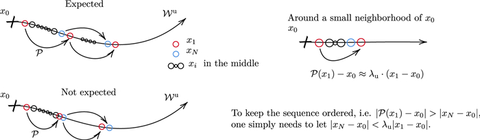
Suppose x₀ is a saddle fixed point of the 2D Poincaré map ${\cal P}$ at an R-Z section. Denote the unstable eigenvalue and eigenvector of ${\cal D}{\cal P}({\boldsymbol{x}_0})$ by λ_u and v_u. If x₀ is instead an m-periodic saddle point, one simply needs to substitute ${\cal D}{{\cal P}^m}({\boldsymbol{x}_0})$ for ${\cal D}{\cal P}({\boldsymbol{x}_0})$. Seed a line of points $\left(\boldsymbol{x}_1, \ldots, \boldsymbol{x}_N\right)$ along v_u, equally spaced, i.e. x_i+1 − x_i is a constant for 0 ≤ i ≤ N − 1. If λ_u ≤ N, ${\cal P}({x_1})$ probably falls behind x_N, i.e. the s of ${\cal P}({x_1})$ is smaller than that of x_N. This makes it difficult to compute s, because the order of s is not certain. Let ${\cal X}$ be a sequence defined by

It is expected that the s of ${\cal P}({\boldsymbol{x}_1})$ should be greater than that of x_N, the s of ${{\cal P}^2}({\boldsymbol{x}_1})$ should be greater than that of ${\cal P}({\boldsymbol{x}_N})$, and so on, i.e. the s of ${{\cal P}^{k + 1}}({\boldsymbol{x}_1})$ should be greater than that of ${{\cal P}^k}({\boldsymbol{x}_N})$, as shown in figure 4. In fact, as long as the s of ${\cal P}({\boldsymbol{x}_1})$ is greater than that of x_N, the conditions for k ≥ 1 are naturally satisfied. Now that ${\cal P}(\boldsymbol{x}) \approx {\boldsymbol{x}_0} + {\lambda _{\rm{u}}}(\boldsymbol{x} - {\boldsymbol{x}_0})$ in the neighborhood of x₀ if x is in the direction of v_u, one simply needs to put x_N closer to x₀ than ${\cal P}({\boldsymbol{x}_1})$, so that $s({{\cal P}^k}({\boldsymbol{x}_N})) < s({{\cal P}^{k + 1}}({\boldsymbol{x}_1}))$. By virtue of this fact, the orbits are untangled with ease and one gets rid of tentative manifold growth methods [11–15], which need to decrease growth step when the local manifold curvature is large. In other words, it is ensured that the sequence

is a strictly increasing sequence, which guarantees that it is safe to compute s by simply accumulating the lengths of segments. Apart from this advantage, this technique to grow manifolds applies to hyperbolic fixed points of n-dimensional maps, $n \in \mathbb{N}^{+}$.

The invariant manifolds in figures 3 and 5 are grown by this naive FLT technique, of which the computed arc lengths s are expressed by the varying color to let it be more easy-to-understand. One can immediately observe that the confinement of this equilibrium relies mostly on the invariant manifolds of the lower X-cycle γ_low, although it also has one X-cycle at top. It is also known as the disconnected double-null configuration.

The blue arrows in figure 5(c) are drawn by the invariant manifold growth formula, which takes ∂X^u/s/∂ϕ and gives ∂X^u/s/∂s. Evidently, ∂X^u/s/∂s is the growth direction of a manifold. The first order central scheme is employed to calculate ∂X^u/s/∂s (s, ϕ) by X^u/s(s, ϕ) at the two neighboring R-Z sections ϕ ± ϵ

4.3.2   Discretizing the invariant manifold growth partial differential equation (PDE) to an ODE system

The other numeric way is to transform the invariant manifold growth formula, a PDE including ∂_s and ∂_ϕ, to a system of ODEs with s as the evolution parameter. Transect the invariant manifold by N R-Z cross-sections at $\left(\phi_i\right)_{i=1}^N$ to discretize it, where $\left(\phi_i\right)_{i=1}^N$ is an arithmetic sequence with a common difference Δϕ = ϕ_i+1 − ϕ_i ranging from 0 to 2mπ − Δϕ. The R and Z coordinates of the manifold at each section contribute two variables of the system, $X_R^{\mathrm{u} / \mathrm{s}}\left(s, \phi_i\right)$ and $X_Z^{\mathrm{u} / \mathrm{s}}\left(s, \phi_i\right)$, totally 2N variables contributed by N sections. Thereafter, $X_R^{\mathrm{u} / \mathrm{s}}\left(s, \phi_i\right)$ and $X_Z^{\mathrm{u} / \mathrm{s}}\left(s, \phi_i\right)$ become univariate functions dependent on s. The manifold growth formula is thereby reduced to a 2N-dimensional ODE system

where Δ X^u/s(s, ϕ_i)/Δϕ denotes a numeric alternative of ∂X^u/s(s, ϕ)/∂ϕ. For example, it can be defined as the first- or second-order central difference schemes

This discretizing method works fine for the invariant manifolds of the outmost saddle cycle(s), but not so for the q = m/n = 3/1 island chain, in which case the four numerically grown invariant branches around an island are almost identical and can not be distinguished as if there were no island there. The primary reason is suspected to be that the two eigenvectors are so close to each other that the grid granularity is not fine enough to distinguish the branch growth directions by finite difference. Although this scheme suffers such a numeric instability, the authors still think it is worth introducing, because this scheme directly utilizes the invariant manifold growth formula and can be useful for those cases that the two eigenvectors of ${\cal D}{{\cal P}^m}$ are not so close.

4.3.3   Denotations and notions explained with the aid of figures

A periodic orbit for a map is best seen as a whole to reflect the intrinsic homoclinic/heteroclinic structure. Then, one can use ${{\cal W}^{\rm{u}}}\left({{\cal P}, \left\{ {{\boldsymbol{x}_1}, {\boldsymbol{x}_2}, {\boldsymbol{x}_3}} \right\}} \right)$ to denote all the unstable branches of the X-cycle of the q = m/n = 3/1 island chain in figure 5. This X-cycle has three strike points $\left\{ {{\boldsymbol{x}_1}, {\boldsymbol{x}_2}, {\boldsymbol{x}_3}} \right\}$ through ϕ = 0 section, each of which has two stable and two unstable branches. Totally there are 6 branches of ${{\cal W}^{\rm{s}}}\left({{\cal P}, \left\{ {{\boldsymbol{x}_1}, {\boldsymbol{x}_2}, {\boldsymbol{x}_3}} \right\}} \right)$ and 6 branches of ${{\cal W}^{\rm{u}}}\left({{\cal P}, \left\{ {{\boldsymbol{x}_1}, {\boldsymbol{x}_2}, {\boldsymbol{x}_3}} \right\}} \right)$. One can also specify a manifold in a more fine-grained way by replacing ${\cal P}$ with ${{\cal P}^m}$, $\left\{ {{\boldsymbol{x}_1}, {\boldsymbol{x}_2}, {\boldsymbol{x}_3}} \right\}$ with x_i, that is ${{\cal W}^{\rm{u}}}\left({{{\cal P}^3}, {\boldsymbol{x}_i}} \right)$ and ${{\cal W}^{\rm{s}}}\left({{{\cal P}^3}, {\boldsymbol{x}_i}} \right)$, which represent the two unstable and two stable branches belonging to the specific point x_i, respectively. Obviously

The 2D manifold ${{\cal W}^{{\rm{u}}/{\rm{s}}}}(\boldsymbol{B}, \gamma )$ consists of all the corresponding 1D manifolds ${{\cal W}^{{\rm{u}}/{\rm{s}}}}({{\cal P}^m}(\phi ), \boldsymbol{x}(\phi ))$ for the Poincaré maps ${{\cal P}^m}(\phi )$ at all sections ϕ, i.e.

where x(ϕ) denotes the (R, Z) coordinates of the cycle γ at ϕ angle, and $\mathcal{P}(\phi): \mathbb{R}^{+} \times \mathbb{R} \rightarrow \mathbb{R}^{+} \times \mathbb{R}$ denotes the Poincaré map at ϕ. where x(ϕ) is a 6π-periodic function representing the (R, Z) coordinates of this X-cycle γ. ${\cal P}({\boldsymbol{x}_0}) = {\boldsymbol{x}_1}$, ${\cal P}({\boldsymbol{x}_1}) = {\boldsymbol{x}_2}$, ${\cal P}({\boldsymbol{x}_2}) = {\boldsymbol{x}_3}$. Then, x(0) = x₁, x(−2π) = x₂, x(–4π) = x₃ (B_ϕ is negative in this shot). Viewing the 3D figure 3 and 2D figure 5 together can help understand the relationship between 2D manifolds ${{\cal W}^{{\rm{u}}/{\rm{s}}}}(\boldsymbol{B}, \gamma )$ and 1D manifolds ${{\cal W}^{{\rm{u}}/{\rm{s}}}}({{\cal P}^m}(\phi ), \boldsymbol{x}(\phi ))$.

In figure 5(b), some regions enclosed by the invariant manifolds of γ_low are filled by colored scatter points. Points are marked with distinctive colors, and then mapped by ${{\cal P}^{ - 1}}$. How these regions are connected by field lines is reflected through the color pattern of scatter points. Let x_low be the strike point of γ_low crossing the ϕ = 0 section. All the points of transversal intersection of the two manifolds ${{\cal W}^{\rm{u}}}({\cal P}, {\boldsymbol{x}_{{\rm{low}}}})$ and ${{\cal W}^{\rm{s}}}({\cal P}, {\boldsymbol{x}_{{\rm{low}}}})$ (the red and blue curves, respectively) are homoclinic to x_low.

Although the fluxes in the colored regions filled by scatter points are the same, e.g. the ① and ② regions in figure 5(b), this flux value probably differs from that of the uncolored regions, e.g. ③ and ④. One should always be careful of this fact.

5.   Discussion and conclusion

5.1   Comparisons with existing works

This subsection compares various approaches developed to study invariant manifolds, albeit obvious. The comparisons of our ${\cal D}{{\cal P}^m}$ evolution and invariant manifold growth formulas with others' works are presented in this subsection subsequently.

Most of existing research has been satisfied with the Floquet's normal form. Floquet theory is so successful that people cease further exploration. Floquet theorem governs how ${\cal D}{\boldsymbol{X}_{{\rm{pol}}}}({\phi _{\rm{s}}}, {\phi _{\rm{e}}})$ varies with ϕ_e. However, it remains unclear how ${\cal D}{\boldsymbol{X}_{{\rm{pol}}}}({\phi _{\rm{s}}}, {\phi _{\rm{s}}} + 2m\pi )$ changes with ϕ_s, which is essential to lessen the computational resources needed to solve for the initial growth directions of stable and unstable manifolds. The most similar work to ${\cal D}{{\cal P}^m}$ evolution formula is given by Tsutumi [38]. Tsutumi considered the following linear system:

where x = x(ϕ, t) is a complex n-column vector and A(ϕ, t) is a complex n × n matrix function T-periodic in ϕ. Theorem 1. in [38] is repeated as below:

There exists a monodromy matrix of (1.1) which does not depend on t⁷ if and only if there exists a matrix function Γ(ϕ, t) which is defined on ∞ < ϕ, t < ∞, T-periodic in ϕ, and satisfies

⁷ In [38], 'there exists a monodromy matrix of (1.1) which does not depend on t′ is equivalent to that 'the internal structure of every monodromy matrix of (1.1) does not depend on t′. By internal structure, Tsutumi means the characteristic multipliers of a matrix and their algebraic and geometric multiplicities.

Tsutsumi's equation (1.2) above is more complicated than our ${\cal D}{{\cal P}^{ \pm m}}$ evolution formula (11) because A(ϕ, t) relies on both ϕ and t. If ∂A /∂t vanishes, one can easily observe that Γ is governed by the same equation as ${\cal D}{{\cal P}^{ \pm m}}$ evolution formula. Tsutsumi did not explain in [38] what Γ can be and how to construct it. His attention was paid to the condition of A(ϕ, t) such that the monodromy matrix does not depend on t. This condition is revealed in his theorem by the existence of the matrix function Γ which satisfies equation (1.2).

The works similar to our invariant manifold growth formula are collated into table 2, in which the work of SS Abdullaev is discussed in the next paragraph and appendix B in more detail. As shown in table 2, the classical invariance equation (1.7) in [10] for n-dimensional maps might be too general for fusion scientists to be useful. TE Evans, JP England, and JM Ottino et al focused on numerical or experimental methods rather than analysis.

Table  2.  Manifold expression comparison.

Method	Manifold and dynamical system dimensions	Typical manifold expression
Ours	2D manifolds of 3D flows	$\frac{\partial \boldsymbol{X}^{\mathrm{u} / \mathrm{s}}}{\partial s}=\frac{\frac{R \boldsymbol{B}_{\mathrm{pol}}}{B_\phi}-\frac{\partial \boldsymbol{X}^{\mathrm{u} / \mathrm{s}}}{\partial \phi}}{ \pm\left\|\frac{R \boldsymbol{B}_{\mathrm{pol}}}{B_\phi}-\frac{\partial \boldsymbol{X}^{\mathrm{u} / \mathrm{s}}}{\partial \phi}\right\|_2}$(16 revisited)
Abdullaev et al	2D manifolds of 3D flows [30]	$\begin{aligned} & F^{(\mathrm{s}, \mathrm{u})}(\phi, x, y)=\gamma x y \\ & \quad \mp \epsilon \frac{\partial}{\partial \phi} P\left(\phi \pm \frac{1}{2 \gamma} \ln \frac{Q}{\gamma|x y|}-\frac{1}{2 \gamma} \ln \left|\frac{x}{y}\right| ; 0\right)=0, \end{aligned}$(70) in [30]
Classical invariance equation	n-D maps [10]	F(W(s)) − W(f(s)) = 0 (1.7) in [10]
Evans et al	2D manifolds of 3D flows [8, 16, 29]	Pure numeric, see section 3 of [29] 'Invariant manifolds associated with a hyperbolic fixed point of the Trip3d_Map, such as ×0 in figure 2, are calculated by constructing the (un)stable eigenvectors $\vec{e}_{(\mathrm{u}), \mathrm{s}}$ associated with a fixed point × and populating a line segment directed along $\vec{e}_{(\mathrm{u}), \mathrm{s}}$ with a set of evenly distributed points'
England et al	1D manifolds of 2D maps [13], 1D manifold of (n − 1)-D Poincaré map induced by n-D flow [14], 2D manifolds of 3D flows [15]	Pure numeric
Ottino et al	2D manifolds of 3D maps [27]	Ottino et al visualized the invariant manifolds schematically by means of a fluid mechanical experiment. In [27], the caption of figure 5.6.3 writes 'Visualization of manifolds Ws(P) and Wu(P) by means of a flow visualization (thought) experiment....'; the caption of figure 5.8.3 writes 'Visualization of manifolds Ws(P) in a time-periodic system by means of a fluid mechanical experiment....'; a sentence around figure 5.8.3 writes 'figure 5.8.3 (which is a continuation of figure 5.6.3) shows, schematically, intermediate times...'

 | Show Table

DownLoad: CSV

Abdullaev [30] has made some contributions to establishing the formula of stable and unstable manifolds. Here we point out the following facts worth noting about his work: (a) his theory relies on the assumption that the perturbation to an axisymmetric magnetic field is small so that the FLT system can be transformed to a perturbed Hamiltonian form; (b) the Poincaré integral is employed to acquire a first order approximation to Poincaré map. By contrast, our Poincaré map is exact; (c) the final formula F^{(s, u)}(ϕ, x, y) = 0 is implicit instead of explicit; (d) the (x, y) coordinates appearing in the formula are not the standard (R, Z) cylindrical coordinates. The x- and y-axes are even probably not perpendicular. A more detailed comparison equipped with equations is put in appendix B.

5.2   Conclusion

Although the magnetic fields in tokamaks are mostly considered axisymmetric, almost all kinds of auxiliary heating schemes, except the ohmic heating of the central solenoid, are strongly localized and non-axisymmetric. The topology of magnetic field plays a dominant role in the behaviour of the confined plasma and the scrape-off layer. Motivated by the curiosity about the intrinsic characteristics of general 3D vector fields (not necessarily divergence-free), an analytic theory on the invariant manifolds of cycles is established in this paper, where the short-period cycles are regarded the skeleton of fields.

The stable and/or unstable manifolds of hyperbolic cycles grow from the eigenvectors of ${\cal D}{{\cal P}^{ \pm m}}(\phi )$. By ${\cal D}{{\cal P}^{ \pm m}}$ evolution formula (11), one gets rid of repetitive 2mπ-integration of equation (3) for ${\cal D}{{\cal P}^{ \pm m}}(\phi )$ at every angle ϕ. The primitive FLT ODE system (1) is extended to the invariant manifold growth formula in cylindrical coordinates (16) by analyzing the relevant differentials.

It is proposed to use the notion of invariant manifolds of outmost saddle cycle(s) to characterize the magnetic topology at the plasma edge when the field is strongly non-axisymmetric. If a tokamak operates in the single-null (respectively double-null, or somehow more strange) mode, there is one (respectively two, or more) outmost saddle cycle(s). The transversely intersecting manifolds are suspected of causing the spiral ribbon-like pattern of heat deposition on the divertor found in tokamak experiments, which needs further verification. In the scrape-off layer, how to disperse the particle and heat fluxes before they land on the divertor is also an interesting problem, worthy of more investigation. With the drift effects taken into account in the future, the heat load pattern observed by diagnostics like infrared thermography is supposed to be more consistent with the divertor regions covered by the invariant manifolds of outmost saddle cycles. For both tokamak and stellarator communities, the transport issue at the plasma boundary is essential to control the heat load below the material limit.

Appendix A.   Proofs

A.1   The geometric meaning of $|{\cal D}{\boldsymbol{X}_{{\rm{pol}}}}({\phi _{\rm{s}}}, {\phi _{\rm{e}}})|$

Proof.

To further simplify the expression above, prepare the following differentials

Reorganize the terms at the right-hand side of equation (A4) in a much more compact way

A.2   ${\cal D}\boldsymbol{X}$ to ${\cal DP}$ formula

C_s and C_e are the matrix $\left[\begin{array}{ccc}\cos \phi & & -R \sin \phi \\ \sin \phi & & R \cos \phi \\ & 1 & \end{array}\right]$ evaluated at the starting and ending points, respectively.

Proof. Consider the differential relationship in cylindrical coordinates

Suppose that the solution $\boldsymbol{X}\left(\boldsymbol{x}_0, t\right)$, crosses the R-Z crosssection $\phi_{\mathrm{e}}$ at the time T. The relevant differentials are related by the equation $\mathrm{d} \boldsymbol{X}\left(\boldsymbol{x}_0, T\right)=\mathcal{D} \boldsymbol{X}\left(\boldsymbol{x}_0, T\right) \cdot \mathrm{d} \boldsymbol{x}_0$ as detailed below

where $\boldsymbol{x}_0$ and $\boldsymbol{X}\left(\boldsymbol{x}_0, T\right)$ denote the starting and ending points, respectively. A similar differential analysis is done for $\boldsymbol{X}_{\mathrm{pol}}\left(\cdot, \phi_{\mathrm{s}}, \phi_{\mathrm{e}}\right)$ as below

The equation above always holds for any $\mathrm{d} x_{0 R}, \mathrm{~d} x_{0 Z}$, and $\mathrm{d} x_{0 \phi}$, hence the corresponding coefficients shall equal

A.3   ${\cal D}{{\cal P}^{ \pm m}}$ evolution formula

Proof. Integrating equation (3) w.r.t. $\phi_{\mathrm{e}}$ from $\phi_{\mathrm{s}}$ to $\phi_{\mathrm{s}}+\Delta \phi$

Differentiating both sides of equation (A18) w.r.t. $\phi_{\mathrm{s}}$

Though it is known how to calculate $\frac{\partial}{\partial \phi_{\mathrm{e}}} \mathcal{D} \boldsymbol{X}_{\mathrm{pol}}\left(\phi_{\mathrm{s}}, \phi_{\mathrm{e}}\right)$ as shown in equation (3), little is known about $\frac{\partial}{\partial \phi_{\mathrm{s}}} \mathcal{D} \boldsymbol{X}_{\mathrm{pol}}\left(\phi_{\mathrm{s}}, \phi_{\mathrm{e}}\right)$. Notice that ${\cal D}{\boldsymbol{X}_{{\rm{pol}}}}({\phi _{\rm{s}}}, {\phi _{\rm{e}}})$ is the inverse matrix of ${\cal D}{\boldsymbol{X}_{{\rm{pol}}}}({\phi _{\rm{e}}}, {\phi _{\rm{s}}})$. The following equation (A23) is useful to solve for $\left(\mathbf{K}^{-1}\right)^{\prime}$ by $\mathbf{K}(x)$ and its derivative $\mathbf{K}^{\prime}(x)$, where $\mathbf{K}(x)$ is a univariate matrix function

Borrow the equation (A23) to solve for $\frac{\partial}{\partial \phi_{\mathrm{s}}} \mathcal{D} \boldsymbol{X}_{\mathrm{pol}}\left(\phi_{\mathrm{s}}, \phi_{\mathrm{e}}\right)$, as shown below

Next, calculate the total derivative of $\mathcal{D} \boldsymbol{X}_{\mathrm{pol}}\left(\phi_{\mathrm{s}}, \phi_{\mathrm{s}}+\Delta \phi\right)$ w.r.t. $\phi_{\mathrm{s}}$. Let $\phi_{\mathrm{e}}=\phi_{\mathrm{s}}+\Delta \phi$

For trajectories of m toroidal turn(s), $\mathbf{A}\left(\phi_{\mathrm{s}}\right)$ and $\mathbf{A}\left(\phi_{\mathrm{s}} \pm 2 m \pi\right)$ are identical since A is a periodic function on the cycle

Let $\Delta \phi$ be $\pm 2 m \pi$, then ${\cal D}{\boldsymbol{X}_{{\rm{pol}}}}({\phi _{\rm{s}}}, {\phi _{\rm{s}}} + {\rm{\Delta }}\phi )$ can be substituted by ${\cal D}{{\cal P}^{ \pm m}}({\phi _{\rm{s}}})$. Equation (A25) is simplified to

One might suspect whether equation (11) works for ${\cal D}{{\cal P}^{ - m}}$, the inverse of ${\cal D}{{\cal P}^m}$. Consider ${\cal D}{{\cal P}^{ - m}} = {({\cal D}{{\cal P}^m})^{ - 1}}$. By equation (A23)

which indicates that the formula (11) applies for both ${{\cal P}^m}$ and its inverse ${{\cal P}^{ - m}}$.

A.4   ${\cal D}{{\cal P}^{ \pm m}}$ eigenvector evolution formula

Proof. Firstly, the eigenvectors are parameterized by θ as shown below

which is safe because, according to the λ-invariance property, the eigenvectors would not become complex on saddle cycles.

Concatenate the two eigenvectors into a matrix V, then

Differentiating equation (A29) w.r.t. ϕ

can be simplified by

Θ and Λ are diagonal and hence commute, therefore equation (A30) becomes

For cycles, $\left(\mathcal{D P}^m\right)^{\prime}=\left[\mathbf{A}, \quad \mathcal{D} \mathcal{P}^m\right]$ implies that $\lambda_1^{\prime}=0, \lambda_2^{\prime}=0$ as shown by the equation (15), then $\boldsymbol{\Lambda}^{\prime}=0$ and equation (A33) is simplified to be

A.5   Invariant manifold growth formula

Proof. The relationship among the differentials ds, dϕ, dR, and dZ is shown in figure A1. To solve for ds/dϕ, the differential ds is given as below

Dividing both sides by $\mathrm{d} \phi^2$

Express the differential $X_R^{\mathrm{u} / \mathrm{s}}(s+\mathrm{d} s, \phi+\mathrm{d} \phi)-X_R^{\mathrm{u} / \mathrm{s}}(s, \phi)$ with ds and dϕ

The Z component $\partial X_Z^{\mathrm{u} / \mathrm{s}} / \partial s$ is similar.

  A1.  Geometric diagram to show the relationship among the differentials ds, dϕ, dR, and dZ. It is supposed that there exists a hyperbolic cycle at bottom, from which an invariant manifold grows. (a) The differential involved in FLT, (b) Two iso-s curves and one iso-ϕ curve of the manifold.

DownLoad: Full-Size Img PowerPoint

Appendix B.   Comparison with Abdullaev's work

Abdullaev firstly transforms the standard cylindrical coordinates (R, Z) to the canonically conjugated variables (z, p_z):

where B₀ is the toroidal magnetic field strength at the major radius R₀, and $\boldsymbol{A}=\left(A_R=0, A_Z, A_\phi\right)$ denotes the vector potential of magnetic field. The normalized poloidal flux ψ_p serves as the Hamiltonian. However, this transform is not always viable when the magnetic field is non-axisymmetric (the definition of ψ_p requires a closed flux surface diffeomorphic to $\mathbb{T}^2$), which limits the application of Abdullaev's method to those near-integrable systems. After that, the FLT equations are presented in the following Hamiltonian form:

A non-axisymmetric magnetic perturbation changes the original axisymmetic poloidal flux $\psi_{\mathrm{p}}^{(0)}$ to:

where ϵ is a dimensionless perturbation parameter dictating the relative strength of perturbation, and $\psi_{\mathrm{p}}^{(1)}\left(z, p_z, \phi\right)$ denotes the perturbation magnetic flux. Such a denotation implies an additional numeric step to transform the perturbation field B_pert(R, Z, ϕ) to $\psi_{\mathrm{p}}^{(1)}\left(z, p_z, \phi\right)$. By comparison, B = B₀(R, Z) + B_pert(R, Z, ϕ) is taken as a whole in our theory, without need to distinguish the perturbation field from the field to be perturbed.

The Poincaré map in [30] is defined to be a full poloidal turn map, with the Poincaré section Σ_s consisting of two segments of the ζ- and η-axes. (ζ, η) is a rectangular coordinate system centered at the X-point (see figure 1 in [30]). Note that ψ_p varies along the ζ-axis. Under the perturbation $\psi_{\mathrm{p}}^{(1)}$, the Poincaré map (ϕ_k, ψ_k) ↦ (ϕ_k+1, ψ_k+1) has the following classical general form:

where the upper and lower signs correspond to the ϕ-increasing and ϕ-decreasing Poincaré maps, respectively. P(ϕ; ψ) is an integral of $\psi_{\mathrm{p}}^{(1)}$ along the unperturbed trajectory, a.k.a. the Poincaré integral

Be careful that the equality of equation (8) only holds when ϵ is infinitesimal, otherwise it is suggested to use ≈ instead of = in equation (8) or add a remainder to for correctness. Equation (8) is the basis for many other equations in [30], which probably also need to change to ≈ when applied to a realistic ϵ.

Let ψ_k+1 = 0 at ϕ_k+1 → ±∞ in equation (8), then Abdullaev immediately obtains the following implicit form of the subset of these two manifolds on Σ_s:

where the upper and lower signs correspond to the stable and unstable manifolds, respectively.

For the points of these two manifolds not on Σ_s, they are mapped to Σ_s along the field lines by equation (36) in [30]. Under the assumption that the magnetic perturbation at the X-point is small and can be neglected, a_x, a_y coefficients in equation (36) are omitted to obtain the following simplified implicit manifold expression:

Note that (x, y) in [30] are not the standard cylindrical coordinates (R, Z), but defined by

where α, β come from the second order term of the expansion of h in the (ζ, η, ϕ) coordinate system

Remind that x- and y-axes are not necessarily perpendicular. The slope of x-axis in (η, ζ) plane is β/α (y = $(-\alpha \xi+\beta \eta) / \sqrt{2 \gamma}=0 \text { on } x \text {-axis }$), while that of y-axis is −β/α ($x=(\alpha \xi+\beta \eta) / \sqrt{2 \gamma}=0$ on y-axis). The product of their slopes equals −β²/α², which does not necessarily equal −1.