Conductivity effects during the transition from collisionless to collisional regimes in cylindrical inductively coupled plasmas

1.   Introduction

Low pressure inductively coupled plasmas (ICPs) are widely utilized for ion sources and material processing. Their popularity for both scientific and industrial applications depends on the capability to achieve high density even for relatively low power and high plasma uniformity, as well as on the possibility of independent control of the ion energy at the plasma boundary.

In the past few decades, substantial experimental and theoretical efforts on the electron kinetics and the electron heating mechanisms have been made in order to understand low pressure ICPs and optimize the discharge characteristics in terms of the individual requirements [1, 2]. The common feature of low pressure ICPs is their non-equilibrium nature. In particular, electrons are not only far from equilibrium with ions and neutrals, but even not in equilibrium within their own ensemble [3]. Non-local electrodynamics and non-local electron kinetics as well as anomalous skin effect and local negative power absorption are distinctive features of the low-pressure regime [4–8]. The differences between non-local electrodynamics and non-local electron kinetics have been introduced in detail by Kolobov et al [8]. The electron energy probability function (EEPF) can deviate from a Maxwellian distribution in these discharges (non-local electron kinetics) [9, 10]. Due to the smaller collision frequency of electrons with neutrals than excitation frequency, the local relation between electron current and electric field (Ohm's law) does not hold true (non-local electrodynamics). In this case, the electron current relies on the distribution of the electric field in the whole plasma and size of the discharge device [11–13]. It is due to the spatial dispersion of conductivity caused by electron thermal motion. Therefore, a non-local conductivity is required to determine the electric field penetration into the plasma.

The accurate description of the discharge properties under low pressures relies on kinetic simulations, where the EEPF, non-local conductivity and plasma density need to be self-consistently calculated. The non-local conductivities for homogeneous plasmas were derived in planar-type [14, 15] and solenoidal-type [16] ICP reactors by Yoon et al. Due to assuming a constant electron density and a Maxwellian EEPF, only the averaged electron Boltzmann equation under linear approximation and the 2D Maxwell equations were solved in their models. Therefore, the interaction between electron properties and electric field cannot be self-consistently considered. Regarding the complexity of theoretical studies in cylindrical geometry, a self-consistent kinetic model with the calculations of nonlocal conductivity, EEPF, and non-uniform profiles of electron density in a one-dimensional (1D) slab geometry was developed by Kaganovich et al [12]. Their model contains the averaged electron Boltzmann equation for EEPF, the Maxwell equation for the electric field, the quasi-neutrality condition for electrostatic potential, and the fluid conservation equations for ion density profile. Subsequently, the kinetic model was used to study the influences of non-local conductivity and non-Maxwellian EEPF on plasma power absorption and plasma density profiles in a 1D planar inductively coupled argon discharge under the non-local regime (pressure ≤10 mTorr) [17, 18]. Recently, Kushner et al reported the influence of non-local conductivity on plasma absorption power in a 2D planar-type argon ICP at 10 mTorr, where electron Monte Carlo simulation instead of electron Boltzmann equation was used to calculate the electron current density [19].

The aforementioned theoretical modellings in the collisionless regime have been well established, while the consideration of inhomogeneous plasmas in a 2D cylindrical geometry is very cumbersome. The fluid equations need to be solved and meanwhile the EEPF as a function of not only the kinetic energy but the potential energy needs to be taken into account. It might limit the studies to some fixed discharge conditions regarding the computational expense. To the best of our knowledge, the effects of plasma conductivity have not been fully reported over a wide pressure range that involves the transition from collisionless to collisional regimes. As mentioned earlier, plasma conductivity couples plasma kinetics to the electromagnetic fields. In this study, a numerical model based on previous work [20] that has been validated is developed to study the conductivity effects during the transition from collisionless to collisional regimes in cylindrical inductively coupled Ar plasmas. In the model, the electron kinetics are addressed by the electron Boltzmann equation, electromagnetic wave properties are obtained by the Maxwell's equations, and plasma density is calculated from global model. The non-local conductivity, local conductivity, and effective conductivity are respectively considered in the model and their effects on plasma parameters and electromagnetic wave characteristics are compared under a wide pressure range of 0.1–20 Pa. The non-local conductivity is computed by the electron Boltzmann equation, while the local conductivity is obtained based on the Ohm's law. The effective conductivity is introduced based on the Ohm's law but with consideration of non-collisional stochastic heating effect by defining a stochastic collision frequency. In principle, the non-local conductivity model should be valid no matter which heating mechanisms (i.e. collisional, collisionless or both of them) dominate the discharge in a given situation.

This manuscript is structured as follows. Section 2 shows a brief description of the model. Verification and validation of the model are shown in section 3. Simulation results and discussions are presented in section 4, where the non-local conductivity effects are compared with local conductivity case and with effective conductivity case. Section 5 presents the conclusions.

2.   Model description

In this work, we consider a cylindrical ICP source with a solenoidal-type coil, and the structure of the chamber is the same as that of the driver chamber of a two-chamber radio-frequency (RF) ICP in the experiments by Li et al [21]. The radius R is 6 cm and the length H is 14 cm. The model is based on the assumption of homogeneous plasma, since the discharge is assumed to be under inductive H mode to produce a thin sheath near the walls.

The model mainly includes three modules of the electron kinetics module (EKM), electromagnetics module (EMM), and global model module (GMM). Harmonic electromagnetic field is generated by the alternating current in the coil by solving the frequency domain wave equation (i.e. EMM), where all physical quantities are assumed to be axisymmetric. For local model, electron current density is obtained based on Ohm's law where the conductivity is local. For non-local model, the determination of electron current density needs a non-local conductivity that is deduced from the EKM (linearized electron Boltzmann equation for perturbed distribution function) with EMM. Electric field from the EMM is used in the EKM (electron Boltzmann equation under quasilinear approximation for isotropic distribution function) to produce normalized EEPF. The normalized EEPF is used to calculate electron impact rate coefficients and other related parameters for the use in the GMM. Particle balance equations for densities of particle species, and power balance equation for density of electrons are solved in the GMM. It is worth noting that only the parts involved in this work as well as variations and improvements in terms of our previous model are shown here and more details can be found in our previous work [20].

2.1   Electromagnetics module

The solution of the inductive electric field can be obtained by the mode analysis method using the Fourier series in a rectangular coordinate system $(x,z)$ [20]

where $k_n$ and ${\mathit{q}}_{\mathit{m}}$ can refer to the previous work [20], and the expansion coefficient $E_{nm}$ of the electric field is given as [20]

where ${\mu }_0,$ $\omega ,$ $I_0,$ $N,$ and $z_k$ are respectively the vacuum permeability, excitation frequency, current amplitude in the coil, number of turns of the coil, and location of the $\mathit{k}\mathrm{th}$ turn in the axial direction. $k_0$ is $\omega /c$ with speed of light c. The conductivity $\sigma$ will be discussed in the EKM.

Based on the solution of electric field, the electron current density $J_{\mathrm{p}}$ can be expressed in terms of $E_y$ via a conductivity $\sigma ,$ and it is given as [20]

2.2   Electron kinetics module

In this part, the non-local conductivity, local conductivity, and effective conductivity, as well as normalized EEPF will be presented.

2.2.1   Non-local conductivity

In the non-local limit, where the electron–neutral collision frequency ${\nu }_{\mathrm{en}}$ is of the same order as (or even smaller than) the excitation frequency $\omega ,$ collisionless heating mechanism might compete with or even dominate over collisional heating in the low-pressure regime. The Ohm's law for electron current density $J_{\mathrm{p}}$ is therefore considered to be not valid anymore. To account for collisionless electron heating, $J_{\mathrm{p}}$ is calculated based on the perturbed distribution function $f_1,$ and it is given by

where $e$ is the elementary charge, $n_{\mathrm{e}}$ is the electron density, and $v_{\mathit{y}}$ is the velocity component in the y direction.

The non-local conductivity can be self-consistently computed by equations (3) and (4). ${\sigma }_n$ is the $n\mathrm{t}\mathrm{h}$ coefficient of non-local conductivity in the Fourier series, and it is given as [20]

where $\epsilon$ is the electron kinetic energy, $m_{\mathrm{e}}$ is the electron mass, $v=\sqrt{2e\epsilon /m_{\mathrm{e}}}$ is the electron velocity, and $f_0$ is isotropic distribution function (i.e. the normalized EEPF). $\mathrm{\Psi }$ and $\mathrm{\Phi }$ can refer to the previous work [20].

2.2.2   Local conductivity

When the electron–neutral collision frequency ${\nu }_{\mathrm{en}}$ is much larger than the excitation frequency $\omega$ at higher pressures, the conductivity is defined by the Ohm's law. It indicates that the collisional heating is the only manner that the electromagnetic field transfers random thermal energy to the plasma. In cases where the local relation between electron current and electric field is valid, the local conductivity for an arbitrary EEPF is given by [17, 22, 23]

2.2.3   Effective conductivity

For the non-local regime, a simpler way to consider the non-collisional stochastic heating is defining an effective conductivity instead of the self-consistent solver of non-local conductivity using electron Boltzmann equation. The collisionless heating in ICPs can be taken into account similar to collisional heating by defining a stochastic collision frequency ${\nu }_{\mathrm{stoc}}.$ In this work, it is determined by ${\nu }_{\mathrm{stoc}}={\overline{\upsilon }}_{\mathrm{e}}/2\pi \delta ,$ where the skin depth is obtained from $\delta ={\left(c^2{\overline{\upsilon }}_{\mathrm{e}}/{\omega }_{\mathrm{pe}}^2\pi \omega \right)}^{1/3}$ [24]. ${\omega }_{\mathrm{pe}}$ is the electron plasma frequency, and ${\overline{\upsilon }}_{\mathrm{e}}$ is the mean velocity of electrons. To take both non-collisional and collisional heating of electrons into account, an effective collision frequency ${\nu }_{\mathrm{eff}}={\nu }_{\mathrm{en}}+{\nu }_{\mathrm{stoc}}$ is defined [1]. Therefore, the effective conductivity by introducing ${\nu }_{\mathrm{eff}}$ instead of ${\nu }_{\mathrm{en}}$ in equation (6) can be written as

The expansion coefficient $E_{nm}$ (see equation (2)) of electric field $E_y$ and electron current density $J_{\mathrm{p}}$ (see equation (3)) mentioned in the EMM are therefore determined based on the three cases of conductivities.

2.2.4   Normalized EEPF

The normalized EEPF $f_0$ can be solved by

where the energy diffusion coefficient $D_{\mathrm{e}}$ is deduced in appendix in detail and is expressed as

$S_0^{(\mathrm{elas})},$ $S_0^{(\mathrm{ex})},$ $S_0^{(\mathrm{iz})}$ and $S_0^{(\mathrm{ee})}$ are the electron–neutral elastic collisions, excitation or de-excitation collisions, ionization collisions and electron–electron collisions [1, 20]. The first three kinds of collision processes are different from our previous work [20], where only the collisions involving the ground state of Ar are considered. In this work, some collisions involving the metastable of Ar are also been included. The term of electron–electron collisions is given as [20]

where the first term on the RHS has the same form as the term on the LHS of equation (8). $D_{\mathrm{ee}}$ and $V_{\mathrm{ee}}$ in equation (10) are respectively given as [25]

where $v_{\mathrm{ee}}$ is the frequency of electron–electron collision [25].

The normalization condition for $f_0,$ ${\displaystyle {\int }_0^{\infty }{f}_0(\epsilon )}{\epsilon }^{1/2}\mathrm{d}\epsilon =1,$ is required. Equation (8) for $f_0$ can be written in the form of an ordinary nonlinear differential equation [25], and solved using the tridiagonal speed-up method.

2.3   Global model module

Global model is also called zero-dimensional model, since it ignores the spatial variation of plasma properties. As known, the global model usually includes particle balance equations for each species except for the background gas, the quasi-neutrality condition, the equation of state for total particle number density, and the power balance equation. Therefore, the global model can be used for the calculation of electron temperature and densities of all particle species. In this study, the normalized EEPF $f_0$ (effective electron temperature $T_{\mathrm{eff}}$ ) is calculated using the electron Boltzmann equation under quasilinear approximation, so the global model is only used for the calculation of the densities of particle species. We discard one of the particle balance equations due to a reduced unknown, i.e. electron temperature in the global model. In our previous work [20], only the power balance equation that is used to determine the electron density is considered. In this work, the particle balance is also included to calculate densities of other particle species, because the Ar metastable is also considered. Even if including Ar metastable has very small effects on the plasma parameters and electromagnetic field properties in this work, the consideration of particle balance equation will help to extend the model to more complex gas discharges for future work. The particle balance equation other than background gas is given as [1, 26]

where $R_{\mathrm{G},i}^{(j)}$ and $R_{\mathrm{L},\mathit{i}}^{(j)}$ are the various creation and loss rates involving species j, respectively. The reaction rate $R_i^{(j)}$ is the product of the densities of reactants and the rate coefficient $k$ of the reaction

where $n_i$ is the density of the ith reactant. For the electron-impact volume reactions, $k$ is calculated based on the normalized EEPF [1]

For the surface reaction for neutrals and positive ions, the rate coefficients can be found in [26]. In this work, the reaction processes of Ar gas are shown in table 1. The cross sections of electron-impact elastic scattering, excitation, de-excitation and ionization are in [27–29].

Table  1.  Reactions considered in the model.

No.	Reaction	Description	Coefficient	Threshold (eV)	References
1	$\mathrm{e}+\mathrm{Ar}\to \mathrm{e}+\mathrm{Ar}$	Elastic scattering	B.E.a	$3m_{\mathrm{e}}{T}_{\mathrm{eff}}/M$	[27]
2	$\mathrm{e}+\mathrm{Ar}\to \mathrm{e}+\mathrm{Ar}*$	Excitation	B.E.	11.6	[28]
3	$\mathrm{e}+\mathrm{Ar}*\to \mathrm{e}+\mathrm{Ar}$	De-excitation	B.E.	-11.6	[28]
4	$\mathrm{e}+\mathrm{Ar}\to \mathrm{e}+{\mathrm{Ar}}^{+}$	Ionization	B.E.	15.8	[27]
5	$\mathrm{e}+\mathrm{Ar}*\to \mathrm{e}+{\mathrm{Ar}}^{+}$	Ionization	B.E.	4.425	[29]
6	$\mathrm{Ar}*+\mathrm{Ar}*\to {\mathrm{Ar}}^{+}+\mathrm{Ar}+\mathrm{e}$	Penning ionization	$1.2\times {10}^{-15}$		[33]
7	$\mathrm{Ar}*+\mathrm{Ar}\to 2\mathrm{Ar}$	Two-body quenching	$2.1\times {10}^{-21}$		[33]
8	$\mathrm{Ar}*+\mathrm{wall}\to \mathrm{Ar}$	Wall recombination	${\left[\frac{{\mathrm{\Lambda }}^2}{D_{\mathrm{Ar}}}+\frac{2V(2-{\gamma }_j)}{A{v}_{\mathrm{Ar}}{\gamma }_j}\right]}^{-1}$		[26]
9	${\mathrm{Ar}}^{+}+\mathrm{wall}\to \mathrm{Ar}$	Wall recombination	$u_{\mathrm{B}}{A}_{\mathrm{eff}}/V$		[26]
aB.E. means Boltzmann equation. The coefficient is calculated based on the integral of the EEPF which is obtained by solving the electron Boltzmann equation.

 | Show Table

DownLoad: CSV

The density of background gas is determined by the equation of state. Meanwhile, the discharge is assumed to satisfy the quasi-neutrality condition. These two criteria are respectively given by

where $T_{\mathrm{gas}}$ is the gas temperature and $k_{\mathrm{B}}$ is the Boltzmann constant. In this work, equation (17) is simplified as $n_{\mathrm{e}}=n_{{\mathrm{A}}_{\mathrm{r}}^{+}}.$

The power balance equation in our previous work [20] is based on the assumption of particle balance by equating the total surface particle loss to the total volume ionization [1]. In fact, it is not quite appropriate, since the EEPF is not strictly Maxwellian and the electron temperature is not determined by the particle balance equation but by the electron Boltzmann equation under quasilinear approximation. It leads to the underestimation of electron density predicted by simulations [20] as increasing pressure when comparing with experiments [21], due to the overestimation of electron loss rate at relatively high pressures. In this work, the power balance equation is utilized in a more general form. The absorption power equals to the bulk power losses caused by electron–neutral collisions, and surface power losses due to charged species flowing to the walls [26]:

where the absorption power $P_{\mathrm{abs}}$ is obtained from the EMM. In this work, we only have one kind of ions, i.e. Ar⁺, so the ion density $n_{\mathrm{i}}$ equals to electron density $n_{\mathrm{e}}.$ $P_{\mathrm{V}}$ is the bulk power loss of an electron per unit volume and $P_{\mathrm{S}}$ is the surface power loss of an ion on the walls per unit volume, respectively. They are given as [26]

where $k_j^{(\mathit{i})}$ is the rate coefficient of ith collision process involving species $j,$ ${\epsilon }_j^{(\mathit{i})}$ is the corresponding threshold energy, and $n_j$ is the number density of neutral particle. The effective area for ions lost to the walls is given as $A_{\mathrm{eff}}=2\pi RL{h}_{\mathrm{R}}/{\mathrm{\Lambda }}_{\mathrm{R}}+2\pi R^2{h}_{\mathrm{L}}/{\mathrm{\Lambda }}_{\mathrm{L}}$ [30, 31]. The mean kinetic energy per electron lost ${\epsilon }_{\mathrm{e}},$ the mean kinetic energy per ion lost ${\epsilon }_{\mathrm{i}},$ and the Bohm velocity $u_{\mathrm{B},i}$ are obtained based on $f_0$ integrals [32].

3.   Verification and validation of the model

3.1   Verification of the model

In order to verify the model, it is compared with the non-local approach to the solution of the Boltzmann equation developed by Kolobov et al [34]. In their work, electron kinetics in a cylindrical ICP sustained by a long solenoidal coil was studied for the near-collisionless regime when the electron mean free path was large compared to the radius of the chamber. For simplicity, they prescribed 1D profiles of the fields and skin depth rather than self-consistently solving the Maxwell equations with electron kinetics and the plasma density. The amplitude of magnetic field ( $B_0$ =2 G), skin depth ( $\delta$ =1 cm) related to plasma density, radius of the chamber (R=5 cm), and RF frequency ( $f$ =13.56 MHz) are the input parameters in their model. The former two quantities are self-consistently calculated in our model. In order to present more reasonable comparison, we try to find the discharge condition capable of making the results of field and plasma density closer to the input ones used in the model of Kolobov et al and the electron mean free path larger than the radius of the chamber [34]. In our simulation, the same radius and RF frequency are used. The length of the chamber is 15 cm, the pressure is 0.5 Pa and the absorption power is 80 W. Under the discharge condition, the calculated skin depth $\delta$ is around 0.95 cm and the amplitude of electric field $E_0$ is 4 V cm^-1 that corresponds to the amplitude of magnetic field $B_0$ of around 1.9 G in our model.

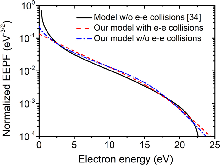
Figure 1 shows that the normalized EEPF predicted by our model is compared with that by the model of Kolobov et al [34]. In their model, the electron–electron collisions were excluded. The normalized EEPFs with and without consideration of electron–electron collisions are predicted by our model. Note that two models achieve reasonable agreement with each other. The model of Kolobov et al predicts a more remarkable depletion at the electron energy higher than 18 eV and more cold electrons with the energy lower than 2.5 eV. The differences between the two models can be due to the different collision processes considered in the two models. The collision processes included in the model of Kolobov et al were not mentioned [34]. If more inelastic collision processes were included in the model of Kolobov et al, it would lead to more depletion in the energetic electrons and enhancement in low-energy ones. As expected, our model without consideration of electron–electron collisions agrees better with the model of Kolobov et al. The inclusion of the electron–electron collisions decreases cold electrons with the energy lower than 2.5 eV, and slightly increases energetic electrons with the energy higher than 18 eV. In general, electron–electron collisions tend to Maxwellize the EEPF.

Figure  1.  Normalized EEPF versus electron energy. Predictions by the model in this work with and without electron–electron collisions and by the model of [34] without electron–electron collisions. Reprinted with permission from [34]. Copyright (1997) by the American Physical Society.

DownLoad: Full-Size Img PowerPoint

In addition, the effects of chamber lengths (i.e. 5, 10, 15, and 20 cm) have also been studied, even if they are not shown here. The simulated EEPF shows that the energetic electrons in inelastic energy range slightly increase with increasing chamber length, because the increased electron energy relaxation length decreases electron energy loss via the inelastic collisions. It leads to slightly higher effective electron temperature at larger chamber length. Shorter chamber length, e.g. 5 cm, makes its scale smaller than the energy relaxation length, but the increased electron–electron collisions due to the increased plasma density still tend to Maxwellize the EEPF. This is because in the model the smaller chamber length produces larger power deposition density and thus higher plasma density for fixed total absorption power.

3.2   Validation of the model

In the previous study [20], the EEPF (electron kinetics) as well as the electron temperature and electron density (basic plasma properties) predicted by the model, was validated with the experiments [21] under the same discharge conditions. Here, we validate the model against experimental measurements in a cylindrical ICP discharge, where the data on electromagnetic wave characteristics under different discharge conditions are available [7]. The experiment is composed of a Pyrex glass tube ( $\mathrm{\Phi }$ 26.3 cm (ID)×45 cm×0.5 cm) and a lower stainless-steel chamber ( $\mathrm{\Phi }$ 45 cm×25 cm×0.5 cm). The ICP source was sustained by a one-turn RF coil made of a copper strip ( $\mathrm{\Phi }$ 32 cm×6 cm×0.05 cm), and the vertical distance between the lower side of the copper strip and the upper side of the stainless-steel chamber was 14.9 cm. The plasma source was shielded with an aluminium cage to suppress RF electromagnetic interference. It is worth noting that the plasma can be very non-uniform especially along the axial direction for this kind of coil position and chamber size. The radial distribution of the RF magnetic field (axial component) was measured using the RF magnetic probe at the center of strip coil along the axial direction. The azimuthal electric field was obtained based on the measured magnetic field.

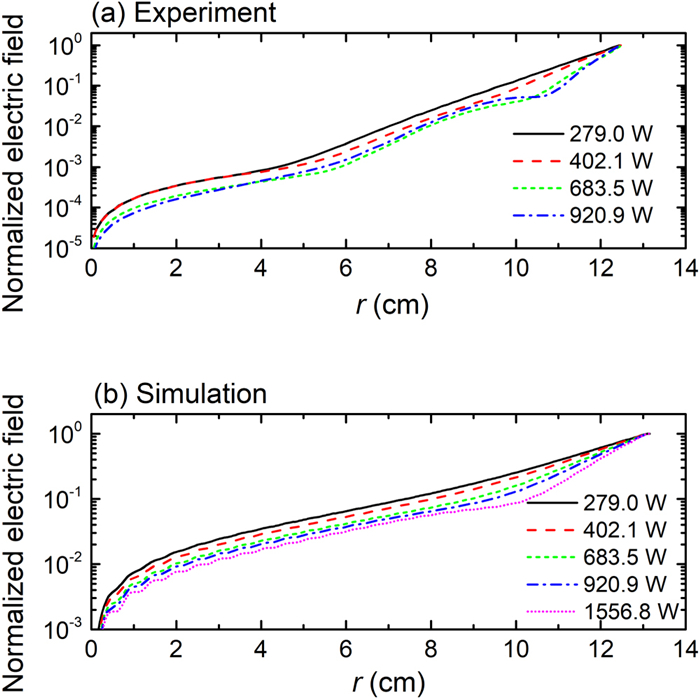
Figures 2(a) and (b) show the 1D radial distributions of electric fields versus power obtained from the experiments and simulations, respectively. Both experiments and simulations show that the electric field rapidly decays from the boundary near the coil to the center of chamber. The electric field decreases faster in the experiment than that in the simulation. This is because the measurements have been performed at the center of strip coil along the axial direction where the plasma density is almost the maximum. Nevertheless, the uniform plasma density assumed in the simulations can possibly make the volume-averaged density smaller than the one in the experiments. Therefore, the lower plasma density in the simulations leads to the deeper penetration and slower decay of the electric field into the plasma. As expected, the lower power facilitates the penetration of electric field into the plasma, which is captured by both simulations and experiments. Note that the higher power produces the non-monotonic field decay, which is typically the anomalous skin effect caused by the collisionless electron thermal motion. The phenomenon has also been observed and discussed in the experiments of an ICP source driven by a planar coil [35]. The non-monotonic evolution of the electric field appears at higher power in the simulation, due to higher power required in the simulation to produce the comparable plasma density to that in the experiment.

Figure  2.  Radial distribution of normalized electric field under different absorption powers at 0.1 Pa. Experimental data (a) reprinted with the permission from [7], copyright (2015), AIP Publishing LLC and predictions by the model in this work (b).

DownLoad: Full-Size Img PowerPoint

4.   Results and discussion

4.1   Non-local conductivity effects

In this section, the effects of non-local and local conductivities on plasma parameters and electromagnetic wave characteristics are compared. The non-local and local conductivities are respectively obtained by solving the electron Boltzmann equation and by using the local approximation. In the simulations, the absorption power is 50 W, the RF excitation frequency is 13.56 MHz, and the pressure varies from 0.1 to 20 Pa. The conductivity is expressed as $\sigma$ in the following figures.

The characteristic lengths play a key role in the definition of non-local and local electrodynamics [8]. If the characteristic size of plasma is much larger than electron mean free path $\lambda$ but is comparable to electron energy relaxation length ${\lambda }_{\epsilon },$ in the collisional (but nonlocal) regime the isotropic part of the electron energy distribution $f_0$ at a given point relies not only on the electric field at this point but also on plasma properties in the vicinity of the point of the size, while the anisotropic part $f_1$ is a local function of the field (i.e. local electrodynamics). If $\lambda$ becomes comparable or even larger than the characteristic size of the plasma. In this nearly collisionless regime, the $f_1$ at a point is determined not only by the local value of the electric field at this point, but also by the profile of the electric field in the vicinity of the point of the size along the electron trajectory (i.e. nonlocal electrodynamics) [8].

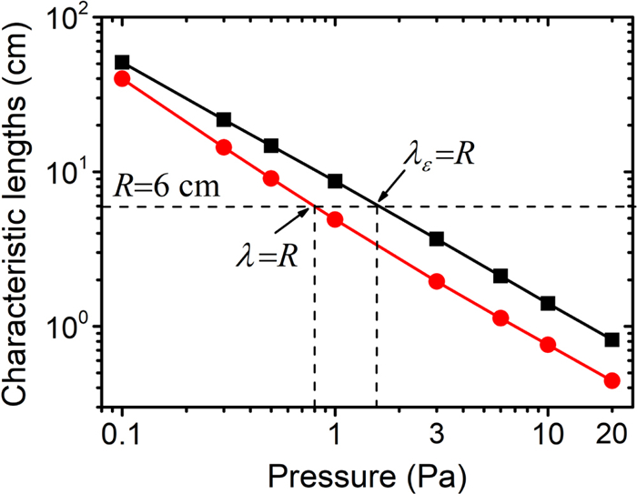
The electron energy relaxation length ${\lambda }_{\epsilon }$ and mean free path $\lambda$ versus pressure are shown in figure 3, and they are compared with the radius of the chamber R. ${\lambda }_{\epsilon }$ is predicted by ${\lambda }_{\epsilon }=\lambda {\left(2m_{\mathrm{e}}/M+{\nu }_{\mathrm{ee}}/{\nu }_{\mathrm{en}}\right)}^{-1/2}$ [1], where $M$ is the argon mass, and ${\nu }_{\mathrm{ee}}$ is the electron–electron collision frequency [25], and the electron mean free path $\lambda ={\overline{u}}_{\mathrm{e}}/{\nu }_{\mathrm{en}}$ with mean electron speed ${\overline{u}}_{\mathrm{e}}$ [1]. At low pressures roughly less than 0.8 Pa where $R<\lambda <{\lambda }_{\epsilon },$ the electrodynamics and electron kinetics are nonlocal. When the pressure is roughly at 0.8 Pa, the mean free path equals to the radius $R=\lambda .$ As slightly increasing pressure (less than roughly 1.6 Pa) where $\lambda <R<{\lambda }_{\epsilon },$ the electron kinetics are nonlocal but the electrodynamics are local. With further increase of the pressures (higher than 1.6 Pa) where ${\lambda }_{\epsilon }<R,$ both the electron kinetics and the electrodynamics are local.

Figure  3.  Electron energy relaxation length and mean free path versus pressure.

DownLoad: Full-Size Img PowerPoint

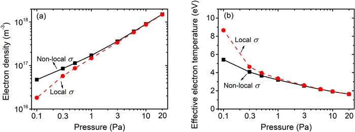
The electron density and effective electron temperature versus pressure under non-local and local conductivities are shown in figure 4. In figure 4(a), electron density monotonously increases with increasing pressure, which achieves qualitatively agreement with the previous experiments [21]. The electron density of non-local conductivity is higher than that of local conductivity at relatively low pressures. It also shows one of the important reasons why the fluid simulation is not valid anymore at very low pressures. The fluid simulations are based on the Ohm's law where only the collisional heating considered is not enough to sustain discharge in low-pressure regime. For example, the electron density of non-local conductivity is far higher than that of local conductivity at 0.1 Pa in our simulation. As increasing pressure, the electron densities under two cases of conductivities tend to converge, which indicates the transition from non-local to local electrodynamics regime. As expected, the effective electron temperature of non-local conductivity is lower than that of local conductivity at relatively low pressures, as shown in figure 4(b). Similar to the variation of electron density, the effective electron temperatures under two cases of conductivities also tend to converge as increasing pressure. The simulation results indicate that the consideration of the non-local conductivity in a low-pressure regime is very important for the development of a numerical model.

Figure  4.  Electron density (a) and effective electron temperature (b) versus pressure under non-local and local conductivities. The excitation frequency is 13.56 MHz and the absorption power is 50 W.

DownLoad: Full-Size Img PowerPoint

The effective electron temperature is obtained based on the integral of normalized EEPF. Figure 5 shows the normalized EEPF versus electron energy at different pressures under non-local and local conductivities. Two cases of conductivities result in a big difference in the normalized EEPF, especially at 0.1 Pa, where the local conductivity produces more electrons in the inelastic energy range and fewer electrons in the elastic energy range. The shape of EEPF is determined by the expansion coefficients in the Fourier series of the electric field, according to equation (9), where the energy diffusion coefficient is proportional to the square of the expansion coefficients of electric field. The effects of collisionless heating under non-local conductivity case allow the electromagnetic wave to couple energy to plasma more efficiently. As a result, the electric field required to deposit a given power into the plasma is smaller than that needed when only considering the collisional heating under local conductivity case. The simulation results of electric fields will be shown later. The stronger electric field under local conductivity case leads to a larger energy diffusion coefficient $D_{\mathrm{e}}$ in the simulations and therefore more energetic electrons penetrate into the RF field region. Consequently, local conductivity produces more electrons in the inelastic energy range.

Figure  5.  Normalized EEPF versus electron energy at different pressures under non-local and local conductivities. The discharge conditions refer to figure 4.

DownLoad: Full-Size Img PowerPoint

In the simulations, the energy diffusion coefficient $D_{\mathrm{e}}$ is smaller than the energy diffusion coefficient related to electron–electron collisions $D_{\mathrm{ee}}$ (see equation (11)) at low electron energy. Therefore, the electron–electron interactions are the only mechanism of energy exchange for the low energy electrons that cannot reach the region of strong electric field where the heating occurs. $D_{\mathrm{ee}}$ under non-local conductivity case is larger than that under local conductivity case due to higher electron density (see figure 4(a)). It leads to more low energy electrons and meanwhile tends to Maxwellize the EEPF in elastic energy range at low pressure of 0.1 Pa under non-local conductivity case. As increasing pressure, the collisionless heating is less efficient and the thermalization of EEPF occurs. The normalized EEPFs evolve into a Maxwellian distribution and are almost identical at 20 Pa for two cases of conductivities. This is because the model-predicted $D_{\mathrm{e}}$ and $D_{\mathrm{ee}}$ for two cases of conductivities are almost the same at 20 Pa.

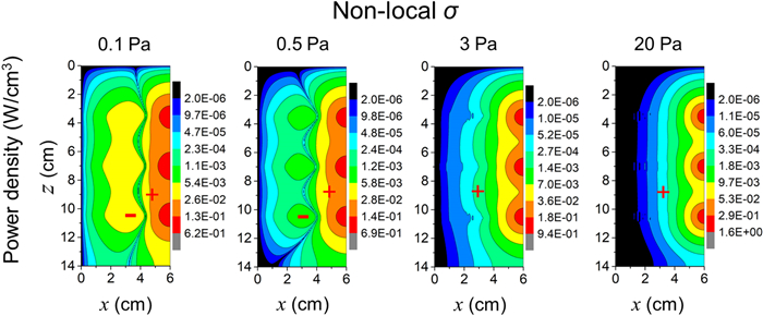
Figure 6 shows the 2D profile of the absorption power density versus pressure under non-local conductivity case. The absorption power density is taken the absolute values and plotted on a log scale to emphasize the negative power absorption. The local negative power absorption in the plasma is predicted by the model with consideration of non-local conductivity at low pressures, for example, 0.1 and 0.5 Pa, and it still exists at 1 Pa even if it is not shown in figure 6. It is well known that the negative power absorption is caused by the thermal motion of electrons. For the case of non-local conductivity, the phase difference between electric field and electron current is not constant. The energetic electrons originating from the discharge edge can be out of phase with an electric field outside the skin layer (close to the center), and lose energy to electric field, thus resulting in negative power absorption. For example, negative power absorption appears close to the discharge center outside the skin layer at 0.1 and 0.5 Pa. The simulation results confirm that there is a spatial region in the discharge where the electrons, instead of taking energy from the field, give back energy to the electromagnetic wave. The size and the number of negative and positive power absorption region depend on the power, which has been experimentally confirmed by Cunge et al [36] and Ding et al [7]. At low power, there is one area of positive and one area of negative power absorption in the radial direction. As increasing power, the number of negative and positive power absorption region increases. Due to a low absorption power of 50 W used in our simulations, there is only one area of positive and one area of negative power absorption.

Figure  6.  2D profiles of absorption power density versus pressure under non-local conductivity. The discharge conditions refer to figure 4. Power density is taken the absolute values and plotted on a log scale to emphasize the negative power absorption.

DownLoad: Full-Size Img PowerPoint

At higher pressures, for example, 3 and 20 Pa, the region of negative power absorption vanishes. It implies that the dominant power transfer mechanism is collisional heating at higher pressures. Even if homogeneous plasma is assumed in the model, the important physical property, i.e. the local negative power absorption, is still captured by the model. It has been demonstrated in the work of Godyak and Kolobov, when comparing the 1D profile of the absorption power density obtained in the experiments with that in the calculation assuming homogeneous plasma [6]. The position and amplitude of positive and negative power densities predicted by the model can be very possibly different from the reality in the experiments where the plasma is inhomogeneous. The uniformity of plasma is better at lower pressure and power. It is well known that the skin depth inversely relies on the electron density [1]. The magnitude and profile of plasma density can affect the magnitude and profile of the electromagnetic fields, electron current, and absorption power density. The absorption power density can be underestimated at the center of the discharge chamber and overestimated at the boundary of the discharge chamber. In addition, the power density profile shrinks and its value becomes larger towards the boundary near the coil, due to the increase in electron density (see figure 4(a)) as increasing pressure.

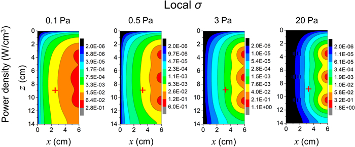
The 2D profile of the absorption power density versus pressure under local conductivity case is shown in figure 7. Very different from the non-local conductivity case, the local negative power absorption is not captured by the local conductivity case at low pressures. For the case of local conductivity, the phase difference between electron current and electric field is constant. Thus, the profile of absorption power relies only on the magnitudes of electric field and local conductivity. At higher pressures, for example, 20 Pa, the 2D profile of the absorption power density under local conductivity case is almost identical with that under non-local conductivity case. It indicates that the collisional heating dominates the discharge at higher pressures. Similar to the non-local conductivity case, the amplitude of absorption power density increases with increasing pressure under local conductivity case due to the increased electron density. As expected, the difference of amplitude in the absorption power density under two cases of conductivities significantly decreases with increasing pressure. For example, for non-local and local conductivities the amplitudes of absorption power density are 0.62 W cm^-3 and 0.28 W cm^-3 at 0.1 Pa and 1.6 W cm^-3 and 1.8 W cm^-3 at 20 Pa.

Figure  7.  2D profiles of absorption power density versus pressure under local conductivity. The discharge conditions refer to figure 4.

DownLoad: Full-Size Img PowerPoint

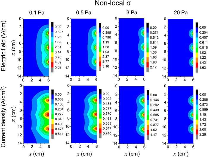
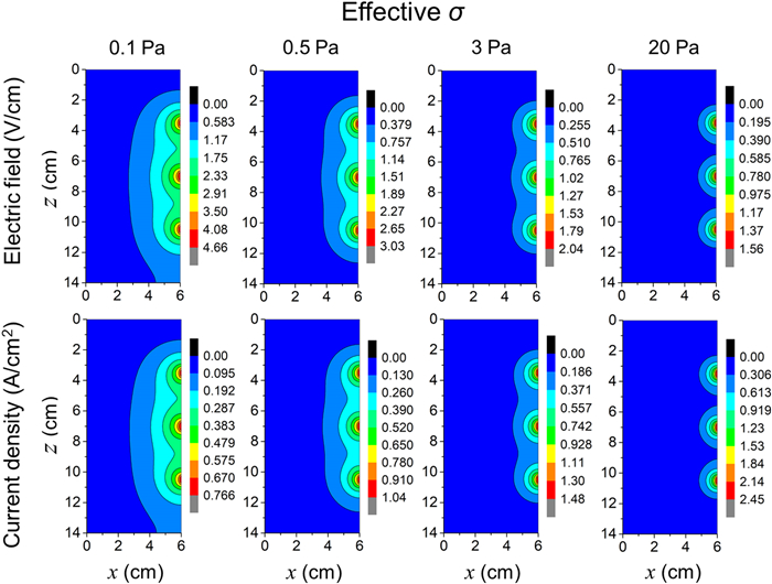
The 2D profiles of electric field and electron current density versus pressure under non-local conductivity are shown in figure 8. As increasing pressure, the 2D profiles of electric field and electron current density shrink towards the boundary near the coil, and the amplitude of the electric field decreases that is consistent with variation of the effective electron temperature with pressure, but the amplitude of the electron current density increases due to the increase in electron density. The non-local relation between electron current density and electric field is more pronounced at lower pressures represented by very different 2D profiles of them. The skin depths $\delta$ predicted by the model are respectively 1.5, 1.0, 0.7 and 0.4 cm at 0.1, 0.5, 3 and 20 Pa. At lower pressures, more electrons contribute to the electron current outside the skin layer and near the plasma bulk, which is a non-local behavior. As increasing pressure, the electron current tends to be determined by the local electric field. Due to homogeneous plasma assumed in the model, the 2D profiles of electron current density and electric field can be slightly different from the reality where the electron density usually has maximum in the discharge center and decreases at the boundary, especially for higher pressures.

Figure  8.  2D profiles of induced electric field (first row) and plasma current density (second row) versus pressure under non-local conductivity. The discharge conditions refer to figure 4.

DownLoad: Full-Size Img PowerPoint

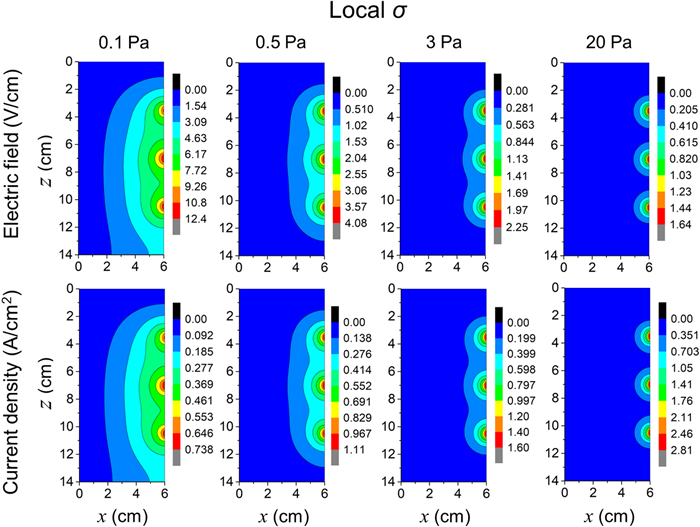
The 2D profiles of electric field and electron current density versus pressure for local conductivity case are shown in figure 9. It is clearly shown that the electron current is determined by the local electric field in the investigated pressure range due to the assumption of Ohm's law between electron current density and electric field. The 2D profiles of electron current density and electric field are identical to each other. The skin depths $\delta$ predicted by the model are respectively 2.3, 1.2, 0.7 and 0.4 cm at 0.1, 0.5, 3 and 20 Pa. Note that $\delta$ under local conductivity case with lower electron density (see figure 4(a)) is larger than that under non-local conductivity case (mentioned in figure 8) at lower pressures. As increasing pressure to 20 Pa, the skin depths are the same (i.e. 0.4 cm) under two cases of conductivities due to the same electron density.

Figure  9.  2D profiles of induced electric field (first row) and plasma current density (second row) versus pressure under local conductivity. The discharge conditions refer to figure 4.

DownLoad: Full-Size Img PowerPoint

The amplitudes of electric field under local and non-local (see figure 8) conductivities are very closer with each other at higher pressures and very different at lower pressures. The amplitude of the electric field under local conductivity case is far higher than that under non-local conductivity case at lower pressures. As mentioned in figure 5, for the case of non-local conductivity the effects of warm-electron and long mean free path cause the electromagnetic wave to couple energy to the plasma more efficiently. The lower electric fields are therefore required to deposit the same total power. It leads to the higher electron density and lower effective electron temperature under non-local conductivity case (see figure 4). For example, at 0.1 Pa, the amplitudes of electric field under local and non-local conductivities are respectively 12.4 V cm^-1 (here) and 5.02 V cm^-1 (see figure 8), therefore the effective electron temperatures are respectively 8.6 eV and 5.4 eV (see figure 4(b)). The consideration of non-local conductivity by solving electron Boltzmann equation in the model is very important for the prediction of non-local relation between electron current and electric field as well as the local negative power absorption in low-pressure regime.

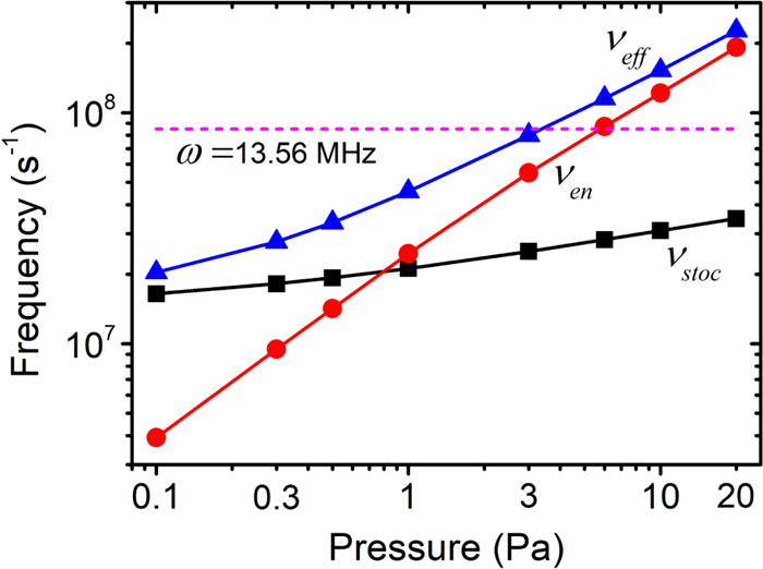
In order to estimate the variation of heating mechanisms with pressure, the characteristic frequencies of plasmas versus pressure are presented in figure 10. These frequencies include electron–neutral collision frequency ${\nu }_{\mathrm{en}},$ stochastic collision frequency ${\nu }_{\mathrm{stoc}},$ and effective collision frequency ${\nu }_{\mathrm{eff}}={\nu }_{\mathrm{en}}+{\nu }_{\mathrm{stoc}}.$ In addition, the value of the excitation frequency $\omega$ is also shown. Both ${\nu }_{\mathrm{en}}$ and ${\nu }_{\mathrm{stoc}}$ are obtained based on the results of the model with consideration of non-local conductivity. The collision frequency ${\nu }_{\mathrm{en}}$ almost linearly increases with increasing pressure because of its proportionality to the density of neutral particles. ${\nu }_{\mathrm{en}}$ is larger than excitation frequency $\omega$ at higher pressures ( $\ge$ 6 Pa), thus the Ohmic heating dominates the discharge. The stochastic collision frequency ${\nu }_{\mathrm{stoc}}$ shows a slight increase with pressure. Comparing ${\nu }_{\mathrm{en}}$ with ${\nu }_{\mathrm{stoc}},$ the Ohmic heating is expected to be dominant at higher pressures as ${\nu }_{\mathrm{en}}$ exceeds ${\nu }_{\mathrm{stoc}}$ by almost one order of magnitude. Due to almost negligible effect of stochastic heating at higher pressures, ${\nu }_{\mathrm{eff}}$ tends to be equivalent to ${\nu }_{\mathrm{en}}.$

Figure  10.  Characteristic frequencies of electrons and excitation frequency $(\omega )$ versus pressure. The characteristic frequencies include the electron–neutral collision frequency $({\nu }_{\mathrm{en}}),$ the stochastic heating frequency $({\nu }_{\mathrm{stoc}}),$ and the effective collision frequency $({\nu }_{\mathrm{eff}}).$ The discharge conditions refer to figure 4.

DownLoad: Full-Size Img PowerPoint

Towards the lower pressures ( $\le$ 3 Pa), the influence of stochastic heating is important. As revealed by the simulation results of absorption power density (see figure 6), the local negative power absorption vanishes at 3 Pa. At 0.8 Pa, ${\nu }_{\mathrm{en}}$ and ${\nu }_{\mathrm{stoc}}$ are the same magnitude. At the lowest pressure limit of 0.1 Pa, because of ${\nu }_{\mathrm{stoc}}$ far higher than ${\nu }_{\mathrm{en}},$ ${\nu }_{\mathrm{eff}}$ significantly deviates from ${\nu }_{\mathrm{en}}$ and tends to be equivalent to ${\nu }_{\mathrm{stoc}}.$ Therefore, the evaluation of the characteristic frequencies shows a transition of the heating mechanism from non-collisional stochastic heating to collision heating as increasing pressure from 0.1 to 20 Pa. It is necessary to consider stochastic heating in low-pressure regime.

4.2   Effective conductivity effects

Due to the importance of collisionless heating caused by the thermal motion of electrons at low pressures, the effective conductivity (equation (7)) is introduced based on the local conductivity (equation (6)) but accounts for the stochastic heating similar to collisional heating by defining a stochastic collision frequency ${\nu }_{\mathrm{stoc}}.$ In order to evaluate the feasibility of effective conductivity at low pressures, its effects on plasma parameters and electromagnetic wave characteristics are compared with non-local conductivity case.

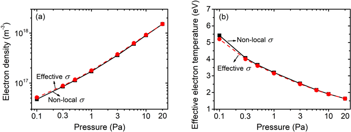
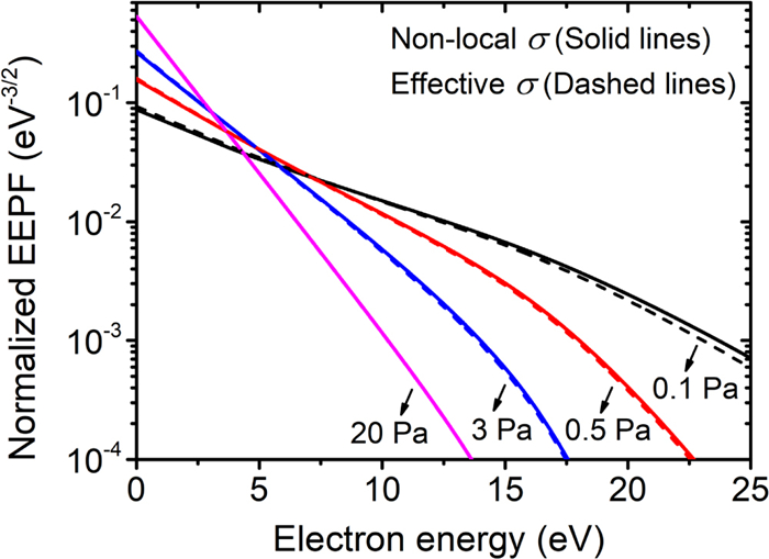
The electron density and effective electron temperature versus pressure under effective and non-local conductivities are shown in figure 11. Different from the comparison between local and non-local conductivities, i.e. figure 4, where very pronounced discrepancies of effective electron temperature and electron density at lower pressures are presented, the effective conductivity almost reproduces the effective electron temperature and electron density under non-local conductivity case in the investigated pressure range. The addition of collisionless heating to collisional heating by introducing the stochastic collision frequency effectively increases electron density compared with the case of only collisional heating taken into account in low-pressure regime. Figure 12 shows the normalized EEPF versus electron energy at different pressures under effective and non-local conductivities. As expected, the normalized EEPF under non-local conductivity case is also almost reproduced by the effective conductivity. It confirms that the effective collision frequency instead of electron–neutral collision frequency taken into account in the solver of local conductivity achieves a more accurate description of electron density and effective electron temperature in low-pressure regime.

Figure  11.  Electron density (a) and effective electron temperature (b) versus pressure under non-local and effective conductivities. The discharge conditions refer to figure 4.

DownLoad: Full-Size Img PowerPoint

Figure  12.  Normalized EEPF versus electron energy at different pressures under non-local and effective conductivities. The discharge conditions refer to figure 4.

DownLoad: Full-Size Img PowerPoint

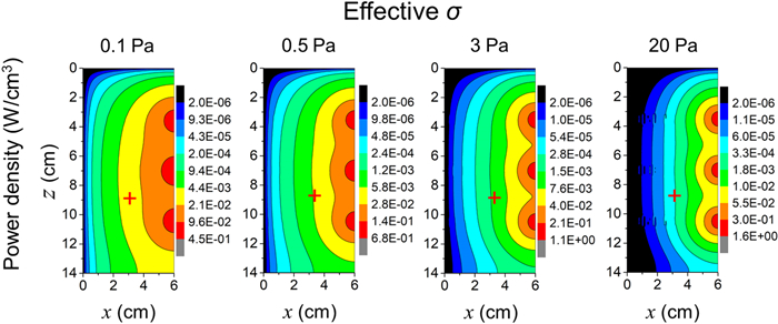
The 2D profile of absorption power density versus pressure under effective conductivity case is shown in figure 13. The effective conductivity almost reproduces the skin depth and the 2D profile of electric field under non-local conductivity case at low pressures of 0.1 and 0.5 Pa, and therefore the effective electron temperature and electron density (see figure 11). However, it does not capture the local negative power absorption that is revealed by the non-local conductivity at low pressures. Meanwhile, the non-local relation between electron current and electric field at low pressures is also not captured by the effective conductivity, as shown in figure 14. This is because despite the effective collision frequency ${\nu }_{\mathrm{eff}}$ instead of the collisional frequency ${\nu }_{\mathrm{en}}$ used in the calculation of conductivity, the determination of electron current density still depends on the Ohm's law. The nature of the local relation between electron current and electric field is not changed for an effective conductivity case.

Figure  13.  2D profiles of absorption power density versus pressure under effective conductivity. The discharge conditions refer to figure 4.

DownLoad: Full-Size Img PowerPoint

Figure  14.  2D profiles of induced electric field (first row) and plasma current density (second row) versus pressure under effective conductivity. The discharge conditions refer to figure 4.

DownLoad: Full-Size Img PowerPoint

5.   Conclusions

Plasma conductivity is a fundamental parameter defining the electrical characteristics of a plasma device. It couples plasma kinetics to electromagnetic fields. In this study, a numerical model for homogeneous plasma is developed to study the conductivity effects in cylindrical inductively coupled Ar discharges at pressures of 0.1–20 Pa. The discharges experience a transition from collisionless to collisional regimes as the pressure increases from 0.1 to 20 Pa. The model consists of an electron kinetics module, electromagnetics module, and global model module. The non-local conductivity, local conductivity, and effective conductivity are respectively considered in the model and their effects on plasma parameters and electromagnetic wave characteristics are compared. The non-local conductivity is addressed by the electron Boltzmann equation. The local conductivity is defined by relating electron current to the electric field using Ohm's law. The effective conductivity is introduced based on the Ohm's law but with consideration of non-collisional stochastic heating effect by defining a stochastic collision frequency.

Simulation results under non-local conductivity cases are first compared with predictions under the assumption of local conductivity case (Ohm's law). The lower effective electron temperature, as well as higher electron density, is obtained for non-local conductivity case than that for local conductivity case at relatively low pressures. This is because the collisionless heating effects under non-local conductivity case allow the electromagnetic wave to couple energy to the plasma more efficiently. Consequently, the electric field required to deposit a given power into the plasma is smaller than that needed when only considering the collisional heating under local conductivity case. The weaker electric field under non-local conductivity case leads to lower effective electron temperature and therefore higher electron density at lower pressures. As increasing pressure, the effective electron temperature and electron density, respectively, tend to converge under two cases of conductivities. It displays a transition of electron kinetics from non-local to local regime. The local conductivity predicts that there is no negative power absorption and the absorption power density monotonically decays from the boundary near the coil towards the discharge center in the investigated pressure range. However, the non-local conductivity predicts a local negative power absorption region and two peaks respectively for positive and negative power absorption regions at relatively low pressures. Almost the same 2D profiles of the absorption power density for non-local conductivity as that for local conductivity are obtained at relatively high pressures. This difference between two cases of conductivities at relatively low pressures can be understood by the prediction of the 2D profiles of electron current density and electric field. More spread-out 2D profile of electron current density than that of electric field under non-local conductivity case indicates a large fraction of electrons coming from the skin layer contributing to the electron current outside the skin layer. The 2D profiles of electron current density and electric field are coincident for local conductivity case in the pressure range of interest, but it only roughly holds true for non-local conductivity case at very high pressure. It verifies that the local relation between electron current and electric field is not valid anymore in the low-pressure regime. The non-local conductivity model is valid no matter which heating mechanisms (i.e. collisional, collisionless or both of them) dominate the discharge in a given situation.

In addition, an effective conductivity with consideration of non-collisional stochastic heating effect is introduced. The effective conductivity almost reproduces the electron density, effective electron temperature, and normalized EEPF under non-local conductivity case in the investigated pressure range. However, the 2D profiles of electric field and electron current density are coincident and there is no negative power absorption in the investigated pressure range. Therefore, the non-local relation between electron current and electric field is not captured by the effective conductivity. This is because the introduction of effective conductivity is still based on the Ohm's law and therefore the nature of the local relation between electron current and electric field is not changed. Even so, for the calculations of effective electron temperature and electron density, the effective conductivity can be alternative to non-local conductivity under the non-local regime in complex modellings such as multi-dimensional fluid simulations for simplicity.

In this work, the effect of the ponderomotive force is not investigated, because it has been proven to be negligibly small at the industrial frequency 13.56 MHz [37]. In future work, the model will be developed to describe the molecular gas discharges, such as hydrogen gas discharge that are extensively used in negative hydrogen ion sources operated at lower RF frequency (1 MHz). In that case, the magnetic (ponderomotive) force can be rather large, because it is almost inversely proportional to the RF frequency [34, 38].

Appendix.   Derivation of the energy diffusion coefficient in the kinetic equation

In order to clarify the derivation of energy diffusion coefficient $D_{\epsilon }$ in equation (8) of the main text, the deduction is shown in detail here. A quasilinear equation for isotropic distribution function $f_0$ is given as [12, 20]

where $\mathit{E}$ and $\mathit{B}$ are respectively the electric field and magnetic field. For arbitrary physical quantities pertaining to simple harmonic oscillation with time $A(t)=A{\mathrm{e}}^{-\mathrm{i}\omega t}$ and $B(t)=B{\mathrm{e}}^{-\mathrm{i}\omega t},$ by averaging their product over the oscillation period $T=\omega /2\pi ,$ we have

Therefore, the kinetic equation for $f_0$ averaged over the RF period is give as

where $f_1(x,z,\mathit{v},t)={\displaystyle {\sum }_{m=1}^{\infty }{\displaystyle {\sum }_{n=-\infty }^{\infty }{F}_{nm}(\mathit{v})\sin ({\mathit{q}}_{\mathit{m}}\mathit{z}){\mathrm{e}}^{\mathrm{i}\left(k_{n}x-\omega t\right)}}}$ [20].

Then, using the orthogonality conditions [20], the kinetic equation for $f_0$ averaged over the space is given as

Because of the commutation relation between the vector $\left({\mathit{E}}_{nm}^{*}+\mathit{v}\times {\mathit{B}}_{nm}^{*}\right)$ and the velocity differential operator ${\mathrm{\nabla }}_{\mathit{v}},$ equation (A4) can be given as

Using ${\mathit{B}}_{nm}=\frac{{\mathit{k}}_n\times {\mathit{E}}_{nm}}{\omega },$ we have

Substituting equation (A6) into (A5), we have

Substituting $F_{nm}(\mathit{v})=\frac{\mathrm{i}e}{m_{\mathrm{e}}}\frac{E_{nm}}{\omega -k_n{v}_x+\mathrm{i}{\nu }_{\mathrm{en}}}·\frac{\partial f_0}{\partial \mathit{v}}$ [20] into equation (A7), we can obtain

where the flux in the velocity space $\mathbf{\Gamma }$ is given as

Using the spherical coordinates in the velocity space

we have

Averaging the ${\mathrm{\nabla }}_v·\mathbf{\Gamma }$ over azimuthal angle in the velocity space, we obtain

where

${\left({\mathit{E}}_{nm}^{*}\right)}_v$ and ${\left({\mathit{k}}_n\right)}_v$ are respectively the projections of ${\mathit{E}}_{nm}^{*}$ and ${\mathit{k}}_n$ in the direction of velocity $\mathit{v},$ and they are given as

Substituting equation (A15) into (A14), we have

where the function $\mathrm{\Psi }$ can be found in [20].

Substituting equation (A16) into (A12) and combining equation (A8), we can obtain

where

For convenience, the RHS of equation (A17) is expressed as a function of energy $\epsilon .$ It is given as

where the energy diffusion coefficient $D_{\mathrm{e}}$ in equation (8) of the main text is obtained as follows

Finally, the effect of magnetic field is cancelled out, because the Lorentz force term ( $\mathit{v}\times \mathit{B}$ ) is averaged over azimuthal angle in the velocity space (see equation (A12)).