Laser-induced breakdown spectroscopy as a method for millimeter-scale inspection of surface flatness

1.   Introduction

Surface flatness is one of the basic geometric tolerances used to evaluate the characteristics of a serving material and the quality of a processing product, and thus, timely inspection thereof plays a key role in many industrial processes [1, 2]. Over the years, various sensors for surface flatness inspection have been developed, and are categorized into two types: contact and non-contact modes. The former is usually based on mechanical principles, and its main advantage is that it can be installed in very harsh environments. However, it cannot be used on very thick or very hot surfaces because the sensor might be damaged [3]. Conversely, the latter is usually based on optical principles, avoiding direct contact of the sensor with the surface, and thus providing the advantage of non-contact optical sensors for high-quality evaluation. It should be noted that the measurement of optical flatness sensors requires two necessary conditions. The surface to be inspected is illuminated by a controlled light source, and the reflected light is collected by a camera, revealing that this type of sensor may not be suitable for the measurement of very bright surfaces [3].

Laser-Induced Breakdown Spectroscopy (LIBS) is an emerging analytical technique to identify and quantify the elements contained in materials by the optical emission of plasma generated by focused laser pulse ablating the material surface (see, for example, references [4‒7]). The attractive advantages of LIBS over traditional techniques include the following: no sample preparation, non-contact detection, real-time and stand-off data collection, almost no destructive effect on the sample. Therefore, LIBS technique provides a good solution for in situ spectrochemical analysis of serving materials or processing products and its application has been accelerated by the development of laser and spectrograph devices at decreased cost, as well as its miniaturization and integration in industrial processes. It should be mentioned that, when LIBS technique is used for spectrochemical analysis, its performance is usually affected by the fluctuation of optical emission of plasma from the material surface with diversity of flatness (hereinafter called flatness effect). Therefore, LIBS-based spectrochemical analysis requires understanding the complexity of the interaction between a focused laser pulse and a material surface exposed to air, especially to determine the LIBS signals complicated by the flatness effect. In fact, previous works [8‒17] have been indirectly focused on the effect investigation using a planished surface of a sample to simulate its various flatness via adjusting the laser Focal plane To the Surface Distance (FTSD). As discussed previously [10‒13], changing the surface flatness (namely, changing the FTSD parameter) leads to a difference in laser spot size on the material surface and therefore to a difference in spatial energy distribution of the laser pulse near and on the surface. This causes a flatness-dependent plasma as an emission source for spectrochemical analysis due to the fact that the laser pulse spatial energy distribution modulated by surface flatness influences the dynamics of plasma generation. As a result, it is expected that the flatness effect, which was originally considered to be an adverse factor for spectrochemical analysis, could possibly be employed to establish a method for inspecting the surface flatness according to certain relationships between the surface flatness and the plasma emission feature that are obtainable from LIBS measurements. Grassi et al have studied the topographic effect related to the differences in the elevation of the sample surface via DP-LIBS. The results demonstrate that the DP-LIBS setup can obtain narrow-scale (approximately micrometer-scale) compositional maps of materials with a lateral depth resolution of micrometer-scale [18]. However, to the best of our knowledge, no one has yet reported a study regarding utilizing this effect for a wide-scale (about millimeter-scale) surface flatness inspection, which could roughly meet the requirements in certain industrial fields [2, 3]. It should be noted that, compared with the case of narrow-scale inspection, there are considerable differences in the flatness-dependent dynamics of laser-induced plasma generation in wide-scale inspection.

In this work, we perform a specific experiment designed to investigate the feasibility of LIBS as an alternative non-contact method for millimeter-scale inspection of surface flatness. The experiment uses a planished alloy steel surface to simulate its various flatnesses via adjusting the FTSD parameter. The obtained results demonstrate that this method is feasible and imply that, for achieving a convenient and wide-range inspection, a multivariate calibration model usually needs to be constructed with the help of machine learning algorithms.

2.   Material and methods

A certified alloy steel with a cylindrical shape (CRM for spectral analysis, CRM-No. GBW01249), which comes from a commercial source (Beijing Zhongke Quality Inspection Biotechnology Co., Ltd.), was selected as a base sample to simulate various surface flatnesses investigated here. The sample dimensions are 30 mm in diameter and 26 mm in height, and its elemental concentrations are listed in table 1. Before performing the LIBS measurements, two flat surfaces of the sample were planished to obtain smooth surfaces with a flatness of about 5 μm.

Table  1.  Certified concentrations of major elements of the alloy steel sample.

CRM-No.	Elemental concentration (wt.%)
	C	Si	Mn	Cr	Ni	W	Fe	Others
GBW 01249	0.582	1.720	1.030	0.301	0.304	1.370	94.502	0.192

 | Show Table

DownLoad: CSV

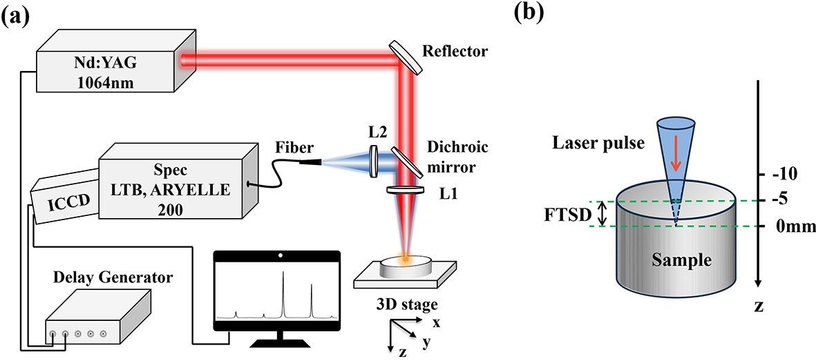
The schematic of the experimental setup is depicted in figure 1(a). A 1064-nm Q-switched Nd:YAG laser (Dawa 300, Beamtech Optronics), operating with 30 mJ pulse energy, 7 ns pulse width and 4 Hz pulse repetition rate, was used as the ablation source. The laser beam with M² factor of about 5 was focused by a 75 mm focal length quartz lens onto the upper flat surface of the sample. A dichroic mirror (Thorlabs, DMLP 900) was used to transmit the laser beam and to reflect the emitted light of the plasma. The emitted light was focused by a quartz lens with a focal length of 75 mm and then transported by a quartz fiber (length: 1.5 m; core diameter: 400 μm), which was fed into an Echelle spectrograph (LTB, ARYELLE 200) equipped with an intensified CCD camera (Andor, DH 334 T). The emission spectra were recorded with a delay time of 1 μs and a gate width of 2 μs. The alloy steel sample was mounted on a 3D translational stage and exposed to air at atmospheric pressure. To refresh the measuring point for each laser pulse, the sample was moved rapidly on the plane perpendicular to the laser beam by the 3D translational stage driven by a miniature reduction motor with extremely small vibration and noise. These experimental operations ensure that each laser shot irradiates a completely fresh surface. To simulate various surface flatnesses, the FTSD parameter was adjusted from −5.0 to −0.6 mm with a step length of 0.2 mm (the negative sign refers to the focal plane below the ablated surface) by moving the sample along the laser propagation direction (see figure 1(b)). These FTSD adjustments simulate various cases of the sample surface flatness (F) ranging from 0 to 4.4 mm when the surface simulated at FTSD = −0.6 mm is used as a reference surface. The laser spot sizes on the surfaces were measured to be about 140 μm at F = 0 mm (FTSD = −0.6 mm) and 340 μm at F = 4.4 mm (FTSD = −5.0 mm), corresponding to the laser irradiances of 27 and 3 GW/cm², respectively. For each simulated case, 66 single-shot spectra were recorded to reduce the statistical fluctuations in the LIBS measurements.

Figure  1.  (a) Schematic of the experimental setup. (b) Definition of the laser focal plane to the surface distance.

DownLoad: Full-Size Img PowerPoint

3.   Results and discussion

3.1   Univariate model for LIBS-based flatness inspection

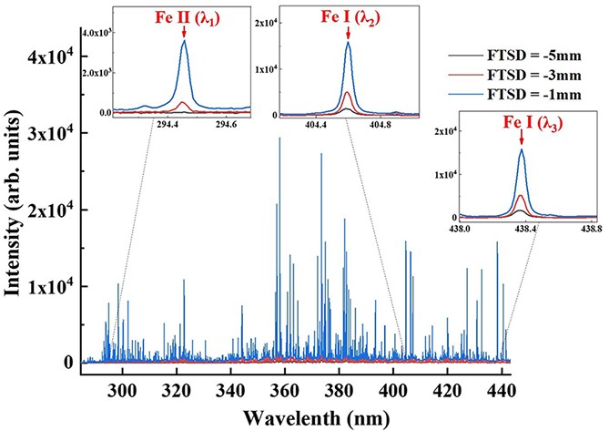
Taking the cases of FTSD = −5 mm, −3 mm and −1 mm (i.e. F = 4.4 mm, 2.4 mm and 0.4 mm) as an example, in figure 2 we show the segment of the LIBS spectra recorded in the wavelength range between 285 nm and 442 nm. Each segment represents an averaged spectrum of 66 single shots. To investigate the feasibility of applying LIBS as a method for inspecting the surface flatness, we chose the three spectral lines at ${\lambda _1}$ = 294.43 nm emitted by single-charged Fe atoms, as well as ${\lambda _2}$ = 404.58 nm and ${\lambda _3}$ = 438.35 nm emitted by neutral Fe atoms as univariate analysis tools for finding flatness indicators. These three lines were chosen because they are present and sufficiently separated in all the FTSD cases involved here. In addition, they have frequently been used in previous LIBS experiments for plasma diagnostic analysis [19‒22].

Figure  2.  LIBS spectra in the wavelength range of 285‒442 nm obtained at FTSD = −5 mm, −3 mm, and −1 mm (F = 4.4 mm, 2.4 mm and 0.4 mm). Three Fe lines selected as univariate analysis tools are enlarged in the insets.

DownLoad: Full-Size Img PowerPoint

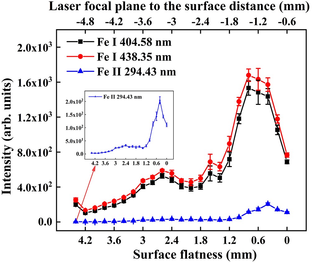
It can be seen that the emission lines obviously depend on surface flatness but the relationship seems to be complicated. To obtain the quantitative dependences, figure 3 shows the emission intensity (I) of each chosen line as a function of F. The I values of the three lines were the average of six spectra generated by 11 single-shot accumulations for each simulated case and were obtained by integrating each spectrum along the line profiles. Indeed, the measured I-F relationships display a complicated flatness effect over the wide F range investigated here, which can be described roughly as follows. For the two atomic lines, with F decreasing, the I values present a slow increase and reach the first extremum at F = 2.6 mm; afterwards, the I values decrease slowly and then surge, reaching the second extremum at F = 0.8 mm followed by a sharp decrease. For the ionic line, the I value presents a very slow increase as F decreases and seems to reach the first extremum at F = 2.4 mm; after that, the I value seems to be constant up to F = 1.4 mm and then surges, reaching the second extremum at F = 0.4 mm followed by a sharp decrease. The measured I-F relationships are consistent with previous investigations [14‒17]. The relationships between I and F are attributed to an extremely complicated multi-factor effect on plasma generation (plasma emission) stemming from the fact that the change in surface flatness leads to simultaneous variations in the laser spot size on the material surface and the laser spatial energy distribution near and on the surface. However, from the perspective of constructing a method for surface flatness inspection via LIBS technique, directly monitoring the variations in spectral intensity seems to be unfeasible to establish a reliable univariate calibration model due to the absence of unambiguous corresponding relationships between I and F.

Figure  3.  Intensities of Fe I lines at 404.58 nm, 438.35 nm and Fe II line at 294.43 nm as a function of surface flatness and laser focal plane to the surface distance. The inset in the left part of the figure shows the enlarged intensities of the Fe II line at 294.43 nm as a function of surface flatness. Error bars correspond to the standard deviations obtained from a series of six spectra generated by 11 single-shot accumulations.

DownLoad: Full-Size Img PowerPoint

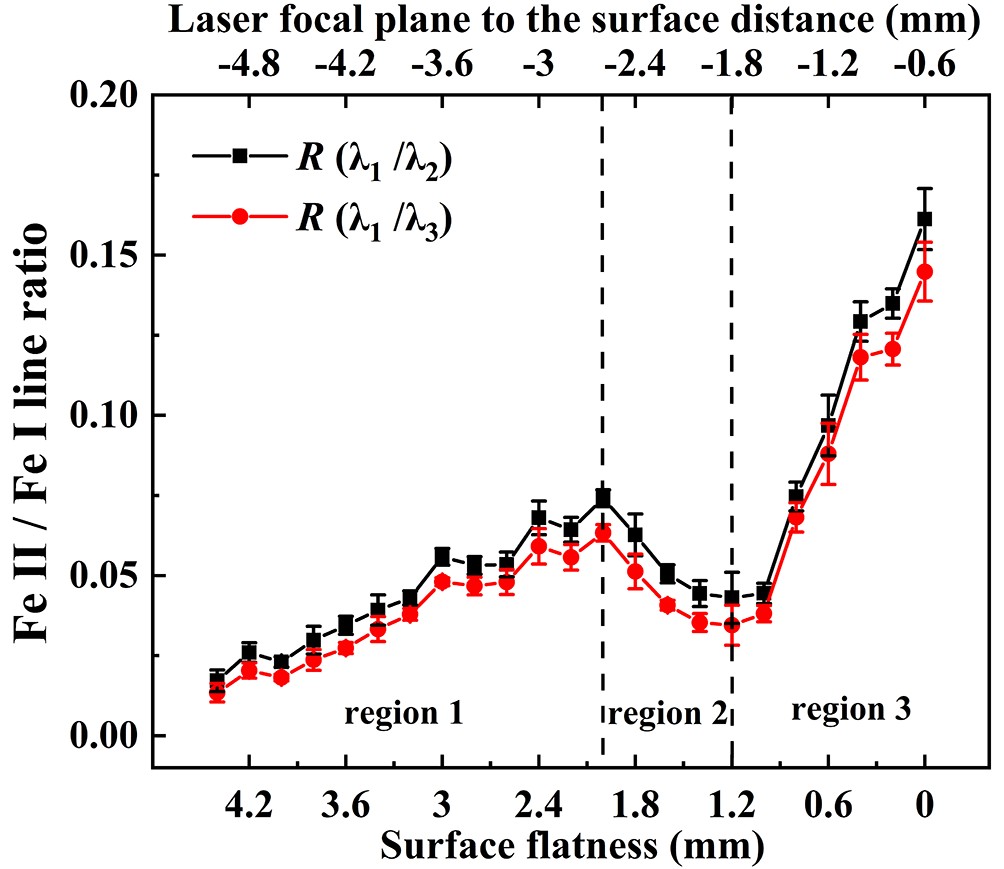
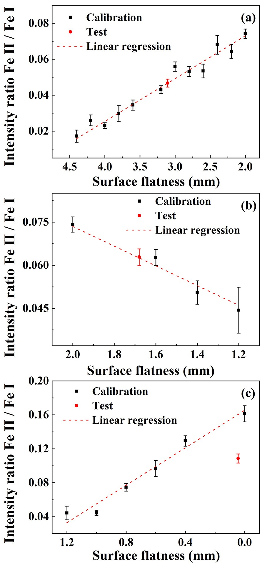
In most of previous LIBS studies that focused on the inspection of material surface hardness [23‒27], the construction of a reliable univariate calibration model is usually based on a linear relationship between the intensity ratio of ionic to atomic lines and the surface hardness. It is interpreted as an effect mediated by laser-induced shock wave. Namely, when the laser irradiance exceeds the sample’s ablation threshold, most of the ablated particles from the surface are still neutral atoms. As the ablated vapor expands, ionization of the ablated atoms occurs directly behind the shock wave front. For a surface with a higher hardness, the shock wave front propagates faster due to a stronger repulsive force on the surface, thus generating a higher temperature region behind the shock wave front and causing an increase in the ionization rate of the ablated atoms located in this region. As mentioned in section 1, changing surface flatness will affect the generation dynamics of laser-induced plasma and certainly affect the front velocity of the concomitant shock wave. Based on this, we examined the evolution of the intensity ratios of Fe II 294.43 nm to Fe I 404.58 nm and Fe II 294.43 nm to Fe I 438.35 nm with surface flatness. Hereinafter, the ratios are noted as $R(\lambda\mathrm{_{II}\mathord{\left/\vphantom{\lambda_{II}\lambda_I}\right.}}\lambda_{\mathrm{I}})$ and their values as a function of F are plotted in figure 4. One can see that the dependences of $R(\lambda_{\mathrm{II}}\mathord{\left/\vphantom{\lambda_{II}\lambda_I}\right.}\lambda_{\mathrm{I}})$ on the surface flatness suggest the identification of three flatness regions, as marked in figure 4, where the flatness effect plays a different role. Specifically, a linear growth of $R(\lambda_{\mathrm{II}}\mathord{\left/\vphantom{\lambda_{II}\lambda_I}\right.}\lambda\mathrm{_I})$ is evident with the decremental F in both regions 1 and 3. However, a near linear decrease of $R(\lambda_{\mathrm{II}}\mathord{\left/\vphantom{\lambda_{II}\lambda_I}\right.}\lambda\mathrm{_I})$ with the decremental F occurs in region 2. This provides direct evidence for the feasibility of inspecting these differences in surface flatness among the “samples” simulated here by selecting the intensity ratio of ionic to atomic lines as a flatness indicator to establish a piecewise univariate calibration model.

Figure  4.  Relationship between the ratios of ionic to atomic line and the surface flatness and laser focal plane to the surface distance. Error bars correspond to the standard deviations obtained from a series of six spectra generated by 11 single-shot accumulations.

DownLoad: Full-Size Img PowerPoint

This feasibility could be well understood by considering the laser-irradiance-dependent plasma generation mechanisms. In a standard LIBS event, the energy of nanosecond laser pulse coupling with the surface usually occurs at the early stage of the plasma formation to generate a cluster of ablation vapor, and the trailing edge of the laser pulse heats the ablation vapor instead of further ablating the surface [28‒31]. Consequently, the status of plasma as an emission source for LIBS measurement is partly determined by the interaction between the vapor and the tailing part of the laser pulse. The interaction mechanisms are frequently described by the laser-supported absorption waves [31‒33], which are divided into two regimes depending on laser irradiance: laser-supported combustion wave (LSCW) at moderate irradiance and laser-supported detonation wave (LSDW) at higher irradiance. In figure 4, region 1 is related to a moderate laser irradiance range (3–9 GW/cm²) due to the larger surface flatness to larger laser spot size on the surface, and therefore an LSCW regime is expected. The main feature of the LSCW regime is that the trailing part of laser pulse can transmit through the ambient air to deposit energy into the ablation vapor. As a result, incremental laser irradiance leads to more energy being deposited into the vapor, resulting in the observed phenomenon of the $R(\lambda_{\mathrm{II}}\mathord{\left/\vphantom{\lambda_{II}\lambda_I}\right.}\lambda_{\mathrm{I}})$ increase with decremental F. In region 2 (laser irradiance range from 9 to 14 GW/cm²), the observed trend reversal of $R(\lambda_{\mathrm{II}}\mathord{\left/\vphantom{\lambda_{II}\lambda_I}\right.}\lambda_{\mathrm{I}})$ with F may imply that a regime transition from LSCW to LSDW occurs. In the laser irradiance range, a new interaction mechanism starts to become important. Specifically, the trailing part of the laser pulse cannot transmit through the ambient air and its energy is effectively absorbed by the ambient air, indicating that in addition to the ablation vapor, a part of the ambient air is also heated directly by the laser pulse. Based on this, it is possible that the temperature of the ablation vapor decreases with the incremental laser irradiance when considering that the mass of the ambient air heated directly by the laser pulse increases rapidly with the incremental laser irradiance. In region 3 (laser irradiance range from 14 to 27 GW/cm²), compared to that in region 1, a faster increase in $R(\lambda_{\mathrm{II}}\mathord{\left/\vphantom{\lambda_{II}\lambda_I}\right.}\lambda\mathrm{_I})$ with decremental F is observed, implying that the interaction mechanism enters the LSDW regime completely. In the laser irradiance range, the mass of ambient air heated directly by the laser pulse does not increase further, indicating that the total mass of the heated ablation vapor and ambient air is almost independent of the laser irradiance. With incremental laser irradiance, the stronger absorption of laser energy by the ambient air leads to the generation of air plasma with a higher temperature and a longer lifetime [30]. The merging between the air plasma and the ablation vapor after a laser pulse may be helpful for maintaining a greater increase rate of the merged plasma temperature with decremental F.

To quantify the feasibility of the method for inspecting the surface flatness via LIBS, a systematic establishment and assessment scheme for the piecewise univariate calibration model (PUCM) will be introduced first. According to the three F regions marked in figure 4, the simulated “samples” were divided into three groups. As shown in table 2, “samples” with surface flatness from 2.0 mm to 4.4 mm, 1.2 mm to 2.0 mm and 0.0 mm to 1.2 mm are named group A, group B and group C, respectively. Furthermore, we select the “samples” with F = 3.4 mm from group A, F = 1.8 mm from group B, and F = 0.2 mm from group C to form a test set for evaluating the generalization performance of the PUCM constructed using the remaining “samples”. Specifically, three evaluation indicators are introduced to assess the PUCM performance as follows: determination coefficient R², relative error of prediction (REP), root mean square error of prediction (RMSEP). Each indicator is calculated by the following equations:

Table  2.  Division of calibration and test sample sets.

Sample groups	Calibration set of samples with F (mm)	Test set of samples with F (mm)
Group A	4.4, 4.2, 4.0, 3.8, 3.6, 3.2, 3.0, 2.8, 2.8, 2.6, 2.4, 2.2, 2.0	3.4
Group B	2.0, 1.6, 1.4, 1.2	1.8
Group C	1.2, 1.0, 0.8, 0.6, 0.4, 0.0	0.2

 | Show Table

DownLoad: CSV

where the index i (= 1, 2, 3, …, n) denotes the calibration “samples” and ${y_i}\left( {{{\hat y}_i}} \right)$ the corresponding reference (predicted) surface flatness of the calibration samples. The index j (= 1, 2, 3, …, m) denotes the test “samples” and ${y_j}\left( {{{\hat y}_j}} \right)$ is the reference (predicted) surface flatness of the test samples. Among these indices, REP(%) and RMSEP reflect the generalization performance of the model. The smaller the REP and RMSEP, the higher the accuracy of the model prediction.

Considering that the dependences of $R\left( {{{{\lambda _1}} \mathord{\left/ {\vphantom {{{\lambda _1}} {{\lambda _2}}}} \right. } {{\lambda _2}}}} \right)$ and $R\left( {{{{\lambda _1}} \mathord{\left/ {\vphantom {{{\lambda _1}} {{\lambda _3}}}} \right. } {{\lambda _3}}}} \right)$ on F presented in figure 4 have similar trends, here only the former was chosen for the establishment and assessment of the PUCM performance. Figure 5 shows the piecewise calibration curves of the PUCM resulted from linear fittings of the intensity ratios of $R\left( {{{{\lambda _1}} \mathord{\left/ {\vphantom {{{\lambda _1}} {{\lambda _2}}}} \right. } {{\lambda _2}}}} \right)$ for the calibration “samples” of group A, group B and group C, respectively. Corresponding test “samples” are then used to evaluate the accuracy of predictions using the established calibration curves. The calculated PUCM performance parameters are summarized in table 3. One can see that, except for the case of group C (R² = 0.911), both group A and group B show an R² value larger than 0.96. It should also be noted that, compared to the cases of both group A and group B (REP = 10.110% and 12.950%), the REP value in group C (45.668%) is not satisfactory. All these values imply that, when intensity ratio $R(\lambda_{\mathrm{II}}\mathord{\left/\vphantom{\lambda_{II}\lambda_I}\right.}\lambda\mathrm{_I})$ is selected as a flatness indicator to establish the PUCM, the model performance seems to have a direct correlation with the regime of the laser-supported absorption because it becomes poor in the LSDW regime.

Table  3.  Parameters indicating the analytical performance of the piecewise univariate calibration model.

F region	R2	REP (%)	RMSEP
2.0‒4.4 mm	0.964	10.110	0.343
1.2‒2.0 mm	0.960	12.950	0.233
0.0‒1.2 mm	0.911	45.668	0.166

 | Show Table

DownLoad: CSV

Figure  5.  Univariate calibration curves [(a) group A, (b) group B, (c) group C] resulted from linear fitting of the intensity ratios $R\left( {{{{\lambda _1}} \mathord{\left/ {\vphantom {{{\lambda _1}} {{\lambda _2}}}} \right. } {{\lambda _2}}}} \right)$ for the “samples” of the calibration set (black squares), and test data (red dots) for each group from the “samples” of the test set.

DownLoad: Full-Size Img PowerPoint

In fact, from practical application perspectives, to achieve a wide range of surface flatness inspections, the use of PUCM inevitably complicates the inspection procedure. To overcome this problem, we tentatively developed a unified multivariate calibration model (UMCM) with the help of back-propagation neural network (BPNN) algorithms. It is expected to be a unified multivariate model for surface flatness inspection within the range of tens to thousands of micrometers using LIBS.

3.2   Multivariate model for LIBS-based flatness inspection

In this section, a BPNN-based UMCM is established to map the relationship between LIBS spectra and corresponding surface flatness, and its performance is presented. According to previous studies [22, 34] devoted to spectrochemical analysis via LIBS, the establishment and assessment schemes of a BPNN-based UMCM mainly include three procedures: data pretreatment, model training, testing. Before these procedures, the same three “samples” as in the case of PUCM establishment (see table 2) were selected as the test set, and the remaining “samples” were used as the training set. In the data pretreatment procedure, first the raw LIBS spectra of the calibration as well as the test sets were normalized with the following formula to reduce the data fluctuation:

where ${I_{ij,{\text{norm}}}}$ represents the normalized intensity of pixel i in the jth spectrum, ${I_{ij,{\text{raw}}}}$ represents the original intensity of pixel i in the jth spectrum and ${I_{j,{\text{min}}}}\left( {{I_{j,{\text{max}}}}} \right)$ is the minimum (maximum) original intensity among the pixels in the jth spectrum.

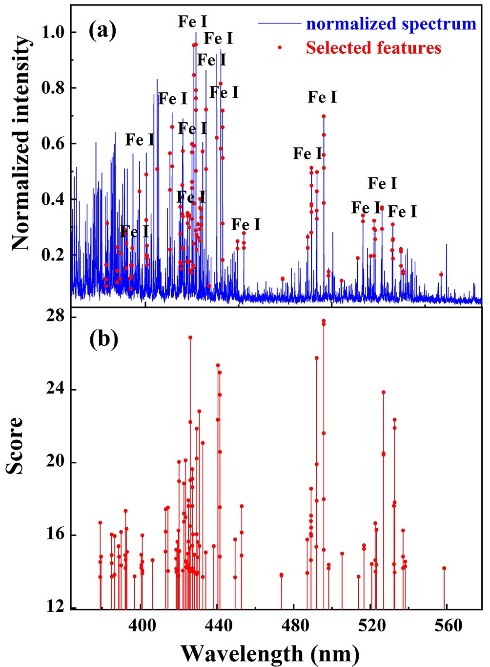
Considering that not all the data in a whole LIBS spectrum are valid for inspecting the surface flatness F, proper data reduction and the selection of significant spectral features are necessary [35, 36]. Since there is a strong correlation between the spectral line intensity and the surface flatness (see figure 3), using the SelectKBest (SKB) algorithm should be most appropriate for feature selection [36, 37]. Following this line, the 150 most significant pixels are selected from the 40995 pixels of normalized spectra of the calibration set as the feature variables to achieve the UMCM establishment. Figure 6 shows the selected features marked on the normalized spectrum obtained at F = 0.4 mm (figure 6(a)) and their corresponding scores (figure 6(b)). One can clearly see that almost all the selected features are distributed on the spectral peaks, especially those from the matrix element Fe.

Figure  6.  Results of spectral feature selection using the SelectKBest algorithm for the flatness inspection. (a) The normalized spectrum (blue line) obtained at F = 0.4 mm and selected 150 pixels (red dots). (b) The scores of the 150 selected features.

DownLoad: Full-Size Img PowerPoint

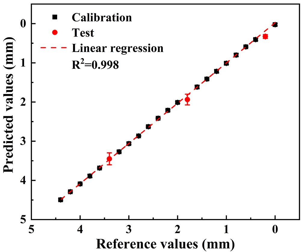
During the model training procedure, a neural network was constructed, which consisted of an input layer with 150 neurons corresponding to the 150 selected features, a hidden layer with 100 neurons and an output layer with a single neuron. Finally, the UMCM performance was tested by importing the test set. During this process, 150 features were selected for each spectrum among the test set using the SelectKBest algorithm and then fed to the UMCM. It needs to be noted that the same three evaluation indicators as in the PUCM case are used to assess the UMCM performance. The values of the three evaluation indicators obtained from training and testing procedures are summarized in table 4, and the surface flatness of the three “unknown” samples predicted using the established UMCM is shown in figure 7 with the multivariate calibration curve.

Table  4.  Parameters indicating the analytical performance of the unified multivariate calibration model.

F region	R2	REP (%)	RMSEP
2.0‒4.4 mm	0.998	3.310	0.132
1.2‒2.0 mm	0.998	6.281	0.152
0.0‒1.2 mm	0.998	15.874	0.127

 | Show Table

DownLoad: CSV

Figure  7.  Multivariate calibration curve (red dashed line) and the predicted values of surface flatness as a function of the certified values of surface flatness of the calibration samples (black squares). Predicted values of surface flatness of the validation samples are indicated by red dots. The error bars are the standard deviations of the replicate measurements for each sample of calibration sets and test sets.

DownLoad: Full-Size Img PowerPoint

It can be seen that the R² value of the UMCM is larger than 0.99, implying a slight improvement relative to the PUCM in the model establishment. To compare its generalization performance with the PUCM, the REP and RMSEP for each test sample were calculated separately. The calculated results show that the values of REP and RMSEP in the three F regions are below 16% and 0.16, respectively, implying a significant improvement in the prediction accuracy compared to the PUCM. These results indicate that a unified calibration model is well established based on BPNN algorithms for unambiguous millimeter-scale range inspection of the surface flatness. It is noteworthy that, although this obtained performance of flatness inspection could roughly meet the requirements in industrial fields, this inspection method may not be suitable in special cases if the roughness of the measured surface is in the order of the spot size.

These performance improvements of a multivariate calibration model compared to a univariate calibration model should be understood as follows. The limitation of univariate models stems from the fact that they only allow for a single independent variable, which greatly constrains the model’s capacity to map the relationship between features and labels. Consequently, univariate models can only accommodate relatively simple mapping relationships, and more complex ones may require a piecewise fitting or may be impossible to fit at all, making them unsuitable for certain types of data analysis, such as surface flatness inspection investigated here. However, the BPNN model employed in this investigation overcomes the limitations of univariate models by utilizing multiple input variables and incorporating numerous hidden nodes. Moreover, the inclusion of activation functions enhances the model’s capacity to handle nonlinear relationships between features and labels [38]. As a result, the neural network model exhibits a powerful fitting ability, surpassing that of univariate models. It should be noted that the established relationships between features and labels are usually affected by inspection conditions. Therefore, sometimes it is necessary to retrain the multivariate model before it is applied to estimate an unknown surface when changing certain inspection conditions, such as laser beam quality.

4.   Conclusion

The purpose of this work is to experimentally investigate the potential of expanding the LIBS application to the inspection of the material surface flatness. This novel application is demonstrated by a specific experiment performed using a planished surface of an alloy steel sample to simulate its various flatnesses, ranging from 0 to 4.4 mm, by adjusting the laser focal plane to the surface distance. We find that the flatness-dependent plasma generation mechanisms play important roles in establishing the method for the LIBS-based flatness inspection. We also find that, to achieve the flatness inspection within a wide range, when univariate analysis is applied, a piecewise calibration model must be constructed. From practical application perspectives, this inevitably complicates the inspection procedure. To solve the problem, we further construct a calibration model based on multivariate analysis and demonstrate that this unified calibration model exhibits favorable performance for unambiguous millimeter-scale inspection of the surface flatness with a resolution of about 0.2 mm. We remark that LIBS combined with machine learning algorithms is a promising tool in real-time measurement of surface flatness, even in simultaneous measurement of certain physical and chemical properties.