Estimating the grain size of microgranular material using laser-induced breakdown spectroscopy combined with machine learning algorithms

1.   Introduction

Randomly packed microgranular (RPMG) materials, such as metal and nonmetal powders, are ubiquitous in industrial activities [1–8]. Grain size significantly affects the structure and properties of RPMG materials and is therefore one of the key physical parameters that need to be monitored to optimize the related industrial processes, especially when they involve the production and application of RPMG materials [9]. There are various methods available for estimating grain size in the range of tens to hundreds of micrometers, for example the sieving method and laser grain size analysis. Although these methods are reliable and effective in most situations, they usually require manual sampling and sample preparation, revealing their intrinsic drawbacks, including being labor-intensive and slow and unsuitable for in situ analysis.

Laser-induced breakdown spectroscopy (LIBS) is an emerging analytical technique for quantifying elements embedded in a material surface by the optical emission of plasma generated by a pulsed laser ablating the surface [10, 11]. The notable advantages of LIBS over common techniques available for elemental analysis, such as secondary-ion mass spectrometry, inductively coupled plasma-optical emission spectroscopy/mass spectrometry and REM-EDX (Raster Electron Microscopic with Energy Dispersive X-ray detection), are suitability for in situ analysis, all-optical contact and real-time data collection. Due to these advantages, LIBS has been extensively used in the fields of public security [12‒14], industrial monitoring [15‒19], deep-sea exploration [20], environmental monitoring [21], etc. Recently, its application as an innovative method for in situ estimation of the surface hardness of a solid material has been constructed and validated [22‒27]. The method was developed in light of the role of shock waves in the expansion of a laser-induced plasma from a solid surface after the end of a laser pulse [28]. Specifically, the speed of the shock wave sufficiently depends on the surface hardness (the higher the hardness, the faster the shock speed). The faster the shock speed, the greater the ionization of the ablated atoms just behind the shock wave during the stage of plasma expansion after the laser pulse. This leads to the widely accepted idea that a univariate calibration model for estimating the surface hardness of solid materials can be established based on the positive relationship between the intensity ratio of ionic to atomic lines and surface hardness. In a recent work [29] the potential of using LIBS to estimate the grain size of RPMG materials within the range from tens to hundreds of micrometers was demonstrated for the first time. The method was developed according to the fact that the grain size affects the mechanical performance of RPMG materials in supporting the recoil stress imparted by the expansion process of laser-induced plasma (hereinafter called laser-induced recoil stress), and therefore affects the formation environment of the luminous plasma. It is worth noting that in the range of grain sizes investigated, completely different dependence behaviors of the plasma formation environment on the grain size occurred in two size regions separated by a critical size [30]. More specifically, when the grain size is above (below) the critical value, the RPMG material has a yield stress larger (smaller) than the laser-induced recoil stress, behaving like an elastic solid (a viscous fluid) to assist (impede) the formation of a luminous plasma with high temperature and high density. This gives rise to the problem that, when univariate analysis is performed, a piecewise univariate model (PUM) has to be constructed in order to estimate the grain size within such wide range. This inevitably complicates the estimation procedure.

To overcome the above problem, in the present work we report a similar experiment to that in [29] but develop a multivariate calibration model with the help of back-propagation neural network (BPNN) algorithms; as a unified multivariate model (UMM) this is expected to replace the PUM constructed previously for estimating the grain size of RPMG materials within the range from tens to hundreds of micrometers using LIBS. Two feature selection strategies with and without considering prior information, respectively, are used to extract useful information from the LIBS data for constructing the UMM. The influence of the feature selection strategy on UMM performance is discussed. A comparison of the performance of PUM and UMM models is provided.

2.   Materials and experiments

2.1   Sample preparation

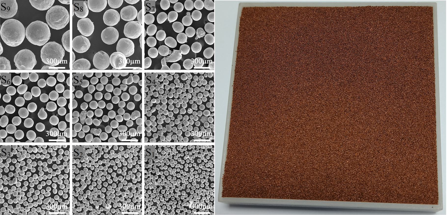
The nine RPMG samples that were used in our previous investigation [29] were also applied in this study. The granular material selected as a base for preparing them is a pile of dry and unconsolidated polydisperse copper microspheres (solid density 8.9 g cm⁻³, purity 99.99%). Specifically, each sample was prepared using a three-step procedure, mainly involving: (1) mechanical sieving with various mesh sizes to obtain nine groups of size-controlled microspheres with a narrow size distribution around the median diameters at 53 (43‒65), 72 (59‒92), 86 (72‒101), 100 (77‒123), 113 (91‒141), 145 (123‒185), 176 (140‒212), 245 (197‒265) and 357 (278‒446) μm, respectively; (2) gently and slowly pouring each group of size-controlled microspheres into the same cubic containers (10 cm inside length); (3) using a straight edge to level each sample surface without any noticeable compaction. The obtained samples and the corresponding SEM images are presented in figure 1. Such a preparation procedure enables the nine prepared RPMG samples (labeled S_n, n = 1‒9 with incremental median diameters) to have the following features: (i) some differences in surface mechanical properties and morphologies mediated only by grain size; (ii) no difference in matrix composition. To ensure experimental reproducibility, after 80 single-shot LIBS measurements made in different spots, each sample in the cubic container was emptied and re-prepared in sextuplicate. Therefore, the changes in LIBS spectra measured under constant experimental conditions among the nine samples are related mainly to their grain sizes.

Figure  1.  Image of a sample and corresponding SEM images. SEM images of the sieved Cu grains used in this study (left). The scale is given in the frames. Sample image taking the case of a median diameter of 72 μm as an example (right).

DownLoad: Full-Size Img PowerPoint

2.2   Setup and data acquisition

A 1064 nm Q-switched Nd:YAG laser (Beamtech Optronics Co., Ltd, Dawa 300), operating with a 7 ns pulse width and 90 mJ pulse energy, was used as the ablation source. The laser beam was focused by a quartz lens with a focal length of 75 mm onto the sample surfaces exposed to air. The sample surfaces were positioned approximately 10 mm closer to the lens than the focal plane and the spot size on the sample surfaces was about 500 μm. A dichroscope (Thorlabs, DMLP 900) was used to transmit the laser beam and to reflect the plasma emission light. The optical emission of the plasma was collected by an optical fiber coupled to an Echelle spectrometer (LTB, ARYELLE 200) and recorded with an intensified charge-coupled device (ICCD; Andor, DH 334T). The gate delay of ICCD detection was set at 1 μs and the gate width was set at 2 μs. Previous work [19] showed that laser ablation of a RPMG sample with fine grains can initiate an excavation process accompanying the ejection of grains. To avoid the influence of excavation on both laser–sample interactions and LIBS measurements of subsequent laser pulses, the laser system worked in 1 Hz mode and the sample was moved rapidly on the plane perpendicular to the laser beam by a mobile platform driven by a miniature reduction motor with extremely low vibration and noise. Such experimental operations ensure that each laser shot irradiates a fresh surface. For more details about the samples and the experimental setup, please refer to our previous publications [29‒32].

3.   Results

3.1   Piecewise univariate model and its performance

As described in the introduction, recent work [29] has demonstrated that the LIBS technique is a feasible method for estimating the median diameter of the nine samples studied here by selecting the plasma temperature (electron density) as a size indicator in the range of median diameter below (above) a critical value of about 110 μm to construct a PUM. It should be noted that a performance analysis of the PUM was not included in the previous work. To facilitate comparisons between the PUM and the UMM to be constructed in the following text, a systematic scheme to assess the performance of the PUM will first be introduced.

In the assessment scheme, according to the critical median diameter (about 110 μm), the nine samples are divided first into two groups: samples S_n (n = 1‒4) with median diameters from 53 to 100 μm and samples S_n (n = 5‒9) with median diameters from 113 to 357 μm, called group A and group B, respectively. Furthermore, we select sample S₂ (72 μm) from group A and S₆ (145 μm) from group B, to form a test set for evaluating the generalization performance of the PUM to be constructed using those remnant samples. Table 1 shows the details of the sample set division. Moreover, the Saha–Boltzmann method and the Stark broadening method are used to calculate the plasma temperature and electron density in laser-induced plasmas. To get a more accurate calculation result, the raw replicate spectra recorded from each sample were respectively averaged. Specifically, an average spectrum was derived from every 80 raw replicate spectra, generating six averaged spectra for each sample. Subsequent calculations of plasma temperature and electron density are based on these averaged spectra.

Table  1.  Sample set division adopted with respect to the piecewise univariate model.

Sample group	Sample set for calibration	Sample set for test
A	S1, S3, S4	S2
B	S5, S7, S8, S9	S6

 | Show Table

DownLoad: CSV

Six evaluation indicators are introduced to assess model performance, as follows: average relative errors of calibration (REC), determination coefficient ${R}^{2}$, slope of the calibration curve, average relative errors of test (RET), relative standard deviations of test (RSD) and root mean square errors of test (RMSET). REC (%) reflects the degree of fitting of the model to the calibration data. RET (%) and RMSET (μm) reflect the generalization performance of the model, with smaller values for both RET and RMSET indicating a higher accuracy of model prediction. RSD (%) represents the stability of the model prediction. Each indicator is calculated by the following equations:

where the index $l$ denotes the $l$th sample for calibration and ${y}_{lk}$(${\hat{y}}_{lk}$) denotes the reference (predicted) median diameter corresponding the $k$th spectrum of the $l$th sample for calibration. The index $p$ denotes the $p$th sample for test and ${y}_{pk}$(${\hat{y}}_{pk}$) denotes the reference (predicted) median diameter corresponding the $k$th spectrum of the $p$th sample for test. $m$ refers to the number of samples in the calibration sample set, $t$ refers to the number of samples in the test sample set and n denotes that each sample corresponds to n averaged LIBS spectra.

The predicted median diameters using the PUM built for sample groups A and B are shown in figures 2(a) and (b), respectively, with a 1:1 curve. We found that, for the calibration sample set, the predicted sizes agree well with the reference sizes, which is in line with the previous results [29]. However, for the test sample set, the predicted sizes deviate obviously from the reference sizes, indicating that the generalization performance of the PUM is not satisfactory. This may be due to various matrix effects and fluctuations of experimental parameters, causing a complex dependence behavior of the plasma temperature (electron density) on the grain size below (above) the critical size.

Figure  2.  (a) Piecewise univariate model for group A. (b) Piecewise univariate model for group B. The black squares represent the calibration samples, the red circles represent the test samples and the blue dotted line is the constructed calibration curve. The error bars are the standard deviations of predicted median diameters. The 1:1 curve is shown as a black line.

DownLoad: Full-Size Img PowerPoint

The quantitative performance of the PUM is summarized in table 2. It can be seen that the determination coefficients of the PUM are greater than 0.9 for both sample groups A and B, and the RET values are 11.12% and 9.67% for groups A and B, respectively. These figures indicate that it is indeed feasible to estimate the median diameter of the RPMG samples in the limited range below (above) the critical size by monitoring the variations in plasma temperature (electron density). It should also be noted from figure 2(b) that the model exhibits a relatively large RSD for samples ${\mathrm{S}}_{8}$ (11.12%) and ${\mathrm{S}}_{9}$ (14.13%), probably indicating that the RET of the model will become poor when predicting unseen grain sizes larger than that of sample ${\mathrm{S}}_{8}$.

Table  2.  Performance of the piecewise univariate model. The definition of groups A and B can be found in table 1.

Sample group	Calibration				Validation
	${R}^{2}$	Slope	REC (%)		RMSET (μm)	RET (%)	RSD (%)
Group A	0.96755	0.96232	4.65		8.00	11.12	3.49
Group B	0.91937	0.97126	6.44		14.02	9.67	3.00

 | Show Table

DownLoad: CSV

3.2   Unified multivariate model and its performance

In this section, a UMM based on the back-propagation neural network (BPNN) algorithm will be built, and its performance presented. Figure 3 provides a visual representation of the step-by-step process for UMM construction, which includes data partitioning, spectral preprocessing, feature selection, hyperparameter optimization through cross-validation and model training. In general, before a UMM is trained, normalization and feature selection are used to reduce high-dimensional LIBS data by extracting useful information from the whole spectrum. Here, the LIBS spectra are normalized with the following formula:

Figure  3.  Flowchart for the buildup of the multivariate calibration model.

DownLoad: Full-Size Img PowerPoint

where ${I}_{ij,\mathrm{n}\mathrm{o}\mathrm{r}\mathrm{m}}$ and ${I}_{ij,\mathrm{r}\mathrm{a}\mathrm{w}}$ represent the normalized intensity and original intensity of pixel $i$ in the $j$th spectrum, respectively. ${I}_{j,\mathrm{m}\mathrm{i}\mathrm{n}}$ (${I}_{j,\mathrm{m}\mathrm{a}\mathrm{x}}$) is the minimum (maximum) original intensity among the pixels in the $j$th spectrum. Following earlier work [22] in which LIBS was combined with machine learning to estimate the physical parameters of materials, the feature is selected according to a linear correlation defined by the following steps as described in [33]:

where index $i$ represents the $i$th pixel, index $j$ represents the $j$th spectrum, N represents a total of N spectra for all samples, $\mathrm{score}_i$ denotes the score of the $i$th pixel, ${I}_{ij}$ denotes the normalized intensity corresponding to the $i$th pixel of the $j$th spectrum, ${S}_{j}$ represents the corresponding median diameter of the $j$th spectrum, ${I}_{i,\mathrm{m}\mathrm{e}\mathrm{a}\mathrm{n}}$ represents the averaged normalized intensity of the $i$th pixel for all samples and ${S}_{\mathrm{m}\mathrm{e}\mathrm{a}\mathrm{n}}$ represents the averaged median diameter for all samples. During the process of feature selection, the pixels with higher scores will be selected as the features of the model.

It should be emphasized that any prior information is not considered in the feature selection process defined by equations (3)‒(7). Here, in constructing the UMM, a novel feature selection strategy will be utilized to extract the useful information from the whole LIBS spectrum according to linear correlation combined with prior information. Such a strategy is also called prior-guided feature selection, similar to that of physics-guided neural networks (PGNNs) [34]. A PGNN is a kind of neural network that uses given laws of physics as constraints to regularize the training process. Such constraints ensure that the learned networks not only admit to lower errors on the training set but also produce predictions that are consistent with the laws of physics. Therefore, in our selection strategy the formula for $\mathrm{score}_i$ and the selection steps are modified as

where ${a}_{i}$ denotes the linear correlation between the normalized intensity of the pixel $i$ and the median diameter of the sample and ${b}_{i}$ denotes the mathematical representation of the prior information, specifically the average normalized intensity corresponding to pixel $i$. The presence of ${b}_{i}$ adds a constraint to the original feature selection: pixels located on characteristic spectral lines are more likely to be used as features. This constraint from the characteristic spectral lines can also be referred to as prior information. Therefore, ${b}_{i}$ represents the prior information. By using a mathematical representation, the prior information is incorporated into the algorithm. ${\lambda }_{a}$ and ${\lambda }_{b}$ are weight parameters that trade off the linear correlation with prior information. It is clear that ${\lambda }_{a}$ = 1 and ${\lambda }_{b}$ = 0 represent the case when prior information is not considered in feature selection.

In addition, hyperparameter optimization was conducted with cross-validation and grid-search parameter tuning. Details can be found in [33]. Specifically, the procedure involves: (1) defining a range and step size for the values of the model hyperparameters (including the number of features); (2) identifying a possible hyperparameter combination and evaluating the associated model performance via cross-validation; (3) systematically exploring all possible combinations of hyperparameters and assessing the corresponding model performance through cross-validation; (4) the hyperparameter combination yielding the optimal model performance is used as the model’s optimal hyperparameters. The optimal hyperparameters used in this work are as follows: the learning rate is 0.005, the batch size is 32, the number of input variables is 100, there is one hidden layer and the number of neurons in the hidden layer is 25. The two test samples defined in groups A and B (see table 1) are merged to produce a test set and the remaining samples are merged to produce a calibration set for UMM construction. The model training process involves multiple iterations, with the aim of optimizing its performance. At the beginning, the weight parameters of the model are randomly initialized, and the selected features are fed into the model to generate prediction results. The predicted values are compared with the reference values, and an error is calculated. Subsequently, the backpropagation algorithm is employed to calculate the gradient of the error with respect to the weight parameters of the model, which are then updated based on this gradient. This iterative process continues until a satisfactory level of accuracy is achieved.

The median diameters of the nine samples predicted using the UMM that was built under the condition of not considering prior information (hereinafter called UMM-1 related to the case of ${\lambda }_{a}$ = 1, ${\lambda }_{b}$ = 0) are shown in figure 4 with a 1:1 curve. One can see that a feasible unified model has been constructed for estimating the grain size of the RPMG samples investigated here via LIBS. For the calibration samples, the predicted sizes agree well with the reference sizes, but for the test samples the predicted sizes deviate obviously from the reference sizes. The quantitative performance of UMM-1 is summarized in table 3. It is found that the RET of UMM-1 is 20.09%, meaning that the generalization performance of UMM-1 is worse than that of the PUM (see table 1). To find out why the performance of UMM-1 becomes worse, the distribution of the corresponding selected features is illustrated in figure 5. Surprisingly, the selected features are distributed in positions with very low normalized intensities (maximum value less than 0.2) instead of on the characteristic peaks of elemental copper. This indicates that the worse performance may be attributed to feature selection without any constraint such as a prior information, meaning that the selected features cannot provide a more appropriate mapping relationship between the LIBS signal and the median diameter.

Figure  4.  The unified multivariate model for ${\lambda }_{a}$ = 1 and ${\lambda }_{b}$ = 0. The black squares represent the calibration samples, the red circles represent the test samples and the blue dotted line is the constructed calibration curve. The error bars are the standard deviations of predicted median diameters. The 1:1 curve is shown as a black line.

DownLoad: Full-Size Img PowerPoint

Figure  5.  The selected features (in red) for ${\lambda }_{a}$ = 1 and ${\lambda }_{b}$ = 0. The raw spectrum (in black) is also shown for comparison.

DownLoad: Full-Size Img PowerPoint

To improve the performance of the UMM, we attempted to construct a UMM with prior-guided feature selection (hereinafter called UMM-2). In the construction process, cross-validation and grid search were used as the optimization techniques to determine the optimal values of ${\lambda }_{a}$ and ${\lambda }_{b}$. After performing a series of procedures, the optimal performance of UMM-2 is achieved when ${\lambda }_{a}$= 0.07 and ${\lambda }_{b}$= 0.93.

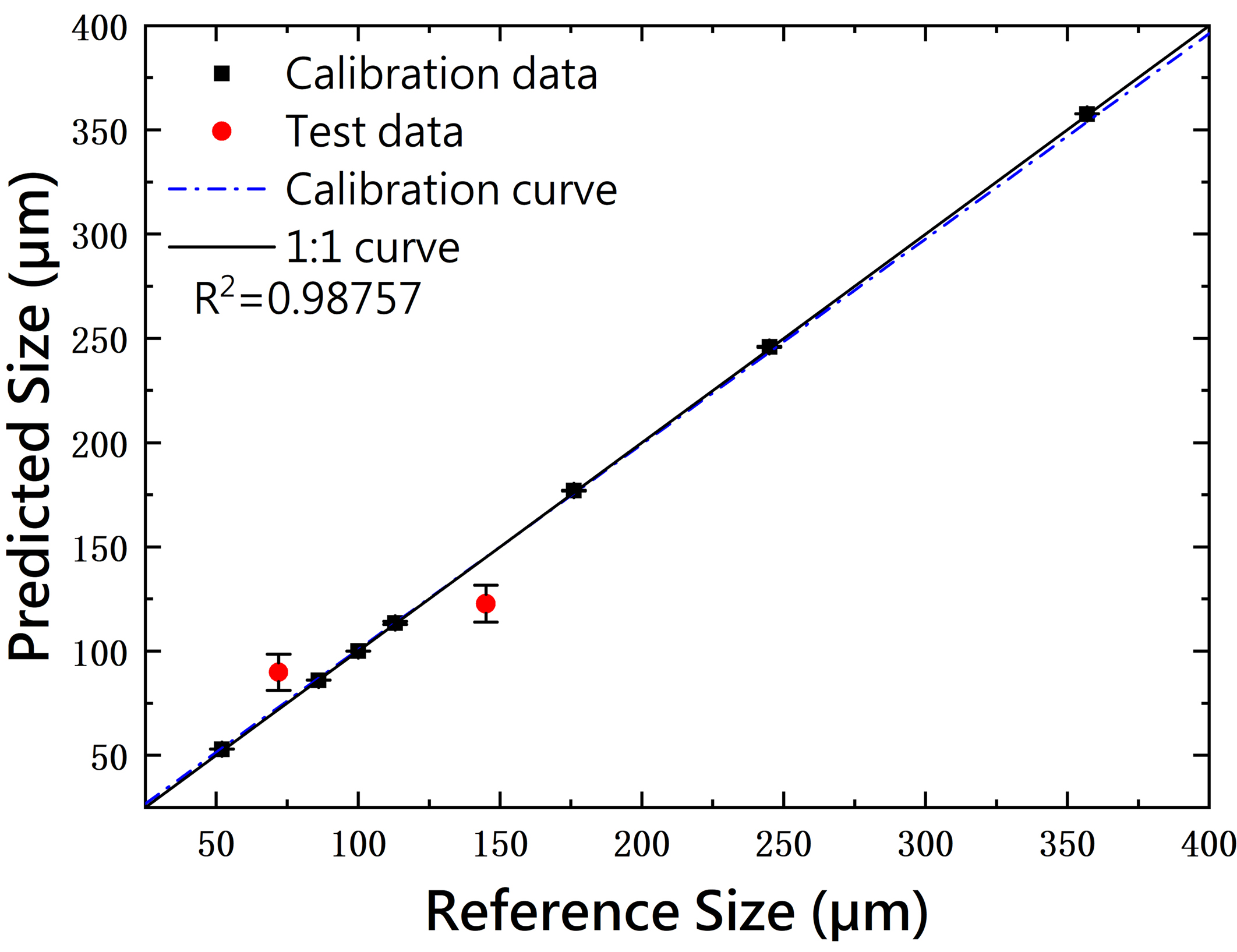
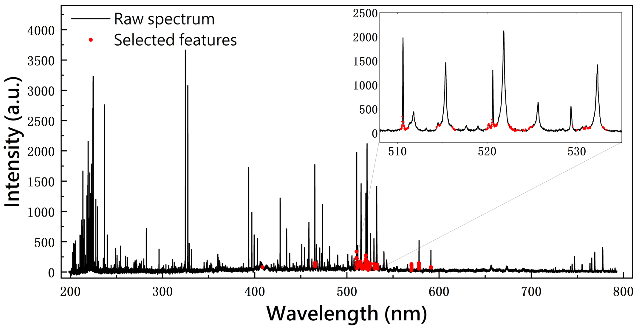
The distribution of the selected features considering prior information (${\lambda }_{a}$ = 0.07, ${\lambda }_{b}$ = 0.93) is presented in figure 6. One can see that most of the selected features are distributed on characteristic peaks of elemental copper, not only the three spectral lines (Cu I 510.6 nm, Cu I 515.3 nm and Cu I 521.8 nm) used to compute plasma temperature and electron density in the PUM but also other lines such as Cu II 427.60 nm, Cu II 458.81nm, Cu II 465.11nm, Cu II 520.71 nm and Cu I 532.37 nm. The median diameters of the nine samples predicted using UMM-2 (${\lambda }_{a}$ = 0.07, ${\lambda }_{b}$ = 0.93) are shown in figure 7 with a 1:1 curve. It is found that the predicted sizes are very close to the reference sizes for the test set. The quantitative performance of UMM-2 is also listed in table 3 (REC = 1.54%, RET = 5.11%), suggesting that an excellent UMM is constructed compared with UMM-1 (RET = 20.09%) and the PUM (RET = 11.12% for group A and RET = 9.67% for group B) for estimating the median diameters of the nine samples investigated here.

Figure  6.  The selected features (in red) for ${\lambda }_{a}$ = 0.07 and ${\lambda }_{b}$ = 0.93. The raw spectrum (in black) is also shown for comparison.

DownLoad: Full-Size Img PowerPoint

Figure  7.  The unified multivariate model for ${\lambda }_{a}$ = 0.07 and ${\lambda }_{b}$ = 0.93. The black squares represent the calibration samples, the red circles represent the test samples and the blue dotted line is the constructed calibration curve. The error bars are the standard deviations of predicted median diameters. The 1:1 curve is shown as a black line.

DownLoad: Full-Size Img PowerPoint

Notably, although the REC of UMM-2 is higher than that of UMM-1, the discrepancy between REC and RET of UMM-2 for the former is less than that for the latter. Such a result should be attributed to the fact that most selected features for the former are distributed on characteristic peaks of elemental copper that aid the establishment of a more appropriate relationship between the LIBS signal and the median diameter.

Table  3.  Performance of the unified multivariate model with different feature selection methods. UMM-1 is the unified multivariate model with $\lambda_a=1\mathrm{\ a}\mathrm{n}\mathrm{d\ }\lambda_b=0$ in the feature selection, and UMM-2 is the unified multivariate model with ${\lambda }_{a}=0.07\;\mathrm{a}\mathrm{n}\mathrm{d}\;{\lambda }_{b}=0.93$ in the feature selection.

Calibration model	Calibration				Validation
	${R}^{2}$	Slope	REC (%)		RMSET (μm)	RET (%)	RSD (%)
UMM-1	0.98757	0.98511	0.25		20.07	20.09	7.31
UMM-2	0.99911	1.00336	1.54		5.61	5.11	4.67

 | Show Table

DownLoad: CSV

4.   Discussion and conclusion

It should be stressed that regardless of whether the prior information is considered in feature selection or not, a UMM can be constructed with the help of BPNN algorithms to estimate the median diameter within the entire size range investigated here (${R}^{2} > 0.98$). This highlights a significant advantage in constructing a unified model using multivariate analysis compared with univariate analysis. The limitation of univariate analysis stems from the fact that it only allows for a single independent variable, which seriously constrains the capacity of the model to fit complex mapping relationships between features and labels. Consequently, univariate analyses only accommodate relatively simple mapping relationships, and more complex ones may require a PUM or even be impossible to construct.

It should also be noted that the performance of a constructed UMM is not always superior to that of a PUM, especially when feature selection is performed without any constraint, such as constraint from prior information. Unconstrained feature selection may result in selected features that encode some of the exclusive information of the calibration set. This ultimately degrades the performance of the model on unseen data. Our results indicate that such an issue may be mitigated when prior information is incorporated as a constraint in the feature selection process. Specifically, the incorporation of prior information may offer more information about the underlying appropriate relationship between features and labels, reducing the risk of overfitting and improving generalization performance to unseen data.

In summary, the most difficult problem in using the LIBS technique to estimate a material parameter is that an appropriate relationship between the LIBS signal and the material parameter has to be established. The present work tells us that this problem can be controlled in a gentle manner once a multivariate model has been constructed using a prior-guided feature selection strategy. This study has practical significance in developing the technology for material analysis using LIBS, especially when the LIBS signal exhibits a complex dependence on the material parameter to be estimated.

Acknowledgments

The authors are grateful to Chen Sun and Jin Yu (Shanghai Jiao Tong University, China) for many scientific discussions and advice. This research was supported in part by the National Key Research and Development Program of China (No. 2017YFA0402300), National Natural Science Foundation of China (Nos. U2241288 and 11974359) and Major Science and Technology Project of Gansu Province (No. 22ZD6FA021-5).